14. L modeling#
14.1. Characteristics of modeling#
Distortion and pure shear in the plane.
|
|
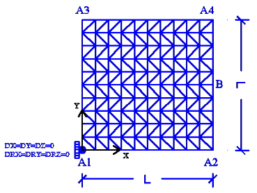
Figure 14.1-a: Meshing and boundary conditions
Modeling: DKTG. \(L=1.0m\).
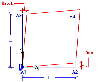
Boundary conditions (see figure above on the right) so that the plate is subject to pure distortion: \({\varepsilon }_{\text{xy}}\) must be constant or to pure shear: forces are applied. Therefore, the following displacement field is applied to the edges of the plate for distortion:
\(\mathrm{\{}\begin{array}{c}{u}_{x}\mathrm{=}{D}_{0}\mathrm{\cdot }y\\ {u}_{y}\mathrm{=}{D}_{0}\mathrm{\cdot }x\end{array}\mathrm{\Rightarrow }\varepsilon \mathrm{=}\frac{1}{2}({u}_{x,y}+{u}_{y,x})\mathrm{=}{D}_{0}\)
So:
we impose an embedding in \({A}_{1}\),
\({u}_{x}={D}_{0}\cdot y,{u}_{y}=0\) on edge \({A}_{1}-{A}_{3}\), \({u}_{x}=0,{u}_{y}={D}_{0}\cdot x\) on edge \({A}_{1}-{A}_{2}\),
\({u}_{x}={D}_{0}\cdot y,{u}_{y}={D}_{0}\cdot L\) on edge \({A}_{2}-{A}_{4}\), \({u}_{x}={D}_{0}\cdot L,{u}_{y}={D}_{0}\cdot x\) on edge \({A}_{3}-{A}_{4}\),
where \({D}_{0}=3.3{10}^{-3}\) and \(f(t)\) represent the magnitude of cyclic loading as a function of the (pseudo-time) parameter \(t\), defined as:
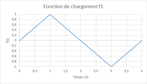
Figure 14.1-b: loading function
Integration increment: \(0.05s\).
For shearing, the following forces are applied:
we impose \({F}_{y}={F}_{0}\) on \({A}_{2}{A}_{4}\),
we impose \({F}_{x}={F}_{0}\) on \({A}_{4}{A}_{3}\),
we impose \({F}_{y}=-{F}_{0}\) on \({A}_{3}{A}_{1}\),
we impose \({F}_{x}=-{F}_{0}\) on \({A}_{1}{A}_{2}\),
with \({F}_{0}=5000000N\)
14.2. Characteristics of the mesh#
Knots: 121.
Stitches: 200 TRIA3; 40 SEG2.
14.3. Modeling DHRC#
Refer to modeling DHRCexpliquée for the H (§ 10) pure traction-compression and I (§ 11) pure flexure models.
14.4. Tested sizes and results#
For the distortion, the shear force \({N}_{\mathrm{xy}}\) and \(B\) obtained by the two models are compared; the tolerances are taken in absolute values based on these relative differences:
Identification |
Reference type |
Reference value |
Tolerance |
DIST. POS .- CHAR. ELAS. \(t=\mathrm{0,25}\) |
|||
Relative difference \({N}_{\mathit{xy}}\) - DHRC - GLRC_DM |
|
-0.171493969414 |
1 10-6 |
DIST. POS. - CHAR. ENDO \(t=\mathrm{1,0}\) |
|||
Relative difference \({N}_{\mathrm{xy}}\) - DHRC - GLRC_DM |
|
-0.151040071429 |
1 10-6 |
DIST. POS. - FROM CHAR. ELAS. \(t=\mathrm{1,5}\) |
|||
Relative difference \({N}_{\mathrm{xy}}\) - DHRC - GLRC_DM |
|
-0.151040071429 |
1 10-6 |
DIST. NEG. - CHAR. ELAS. \(t=\mathrm{3,0}\) |
|||
Relative difference \({N}_{\mathrm{xy}}\) - DHRC - GLRC_DM |
|
-0.151040071429 |
1 10-6 |
DIST. NEGNEG. ATIVE - DECHAR. ELAS . \(t=\mathrm{3,5}\) |
|||
Relative difference \({N}_{\mathrm{xy}}\) - DHRC - GLRC_DM |
|
-0.151040071429 |
1 10-6 |
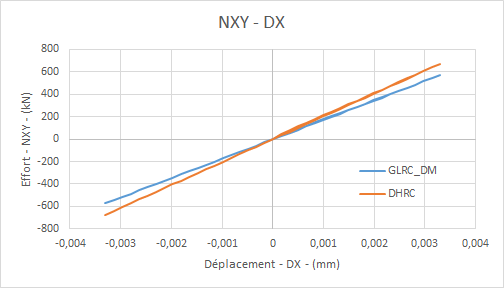
Shearing force diagram \({N}_{\mathit{xy}}\) (in the plan) as a function of time:
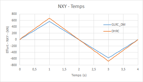
shear force graph \({N}_{\mathit{xy}}\) **** (in the plan) **based on:math:`{D}_{0}`**imposed: **
For shear, we do non-regression tests on shear deformations \({\epsilon }_{\mathit{xy}}\) and \(B\):
Identification |
Reference type |
Reference value |
Tolerance |
|
CISAIL. POS. - ELAS . \(t=\mathrm{0,1}\) |
||||
\({\epsilon }_{\mathit{xy}}\) - GLRC_DM |
|
4.7587148531429.10-4 |
1 10-6 |
|
CISAIL. POS. - ENDO . \(t=\mathrm{0,8}\) |
||||
\({\epsilon }_{\mathit{xy}}\) - GLRC_DM |
|
9.09169470373.10-3 |
1 10-6 |
|
CISAIL. POS. - ELAS . \(t=\mathrm{0,1}\) |
||||
\({\epsilon }_{\mathit{xy}}\) - DHRC |
|
1.78152989856.10-4 |
1 10-6 |
|
CISAIL. POS. - ENDO . \(t=\mathrm{0,8}\) |
||||
\({\epsilon }_{\mathit{xy}}\) - DHRC |
|
1.93228925951.10-3 |
1 10-6 |
1 10-6 |