10. H modeling#
10.1. Characteristics of modeling#
Pure Traction - Compression.
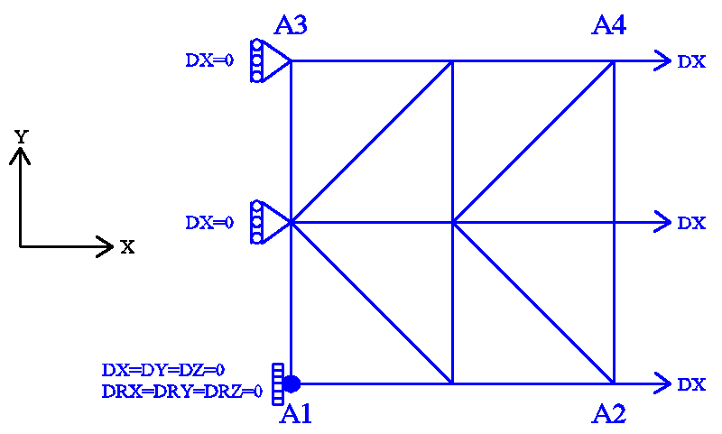
Figure 10.1-a: mesh and boundary conditions.
Modeling: DKTG
Boundary conditions:
Embedding in \({A}_{1}\);
\(\mathrm{DX}=0.0\) on the \({A}_{1}-{A}_{3}\) edge;
\(\mathrm{DX}={U}_{0}\times f(t)\) on the \({A}_{2}-{A}_{4}\) edge;
where \({U}_{0}=1.0\times {10}^{-3}m\) and \(f(t)\) represent the amplitude of cyclic loading as a function of the (pseudo-time) parameter \(t\). To properly verify the model, we consider a loading function as follows:
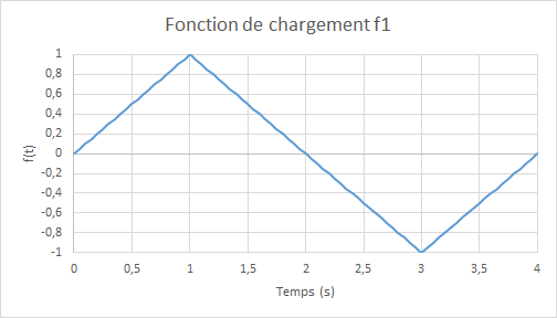
Figure 10.1-b: loading function: traction, then compression
Note: the extreme deformation is: \(1.0\times {10}^{-3}\) , or about a third of the deformation during the transition to plasticity of steels. No integration time: \(0.025s\) .
10.2. Characteristics of the mesh#
Number of knots: 9.
Number of stitches: 8 TRIA3; 8 SEG2.
10.3. Modeling DHRC#
The models corresponding to high stress levels allow the validation of model DHRC. This model is in fact able to represent the relative slip between the reinforcing bars and the surrounding concrete during high levels of stress. H modeling then compares the results obtained for model DHRC with those of models GLRC_DM and EIB. The parameters chosen for GLRC_DM are then adjusted according to the parameters identified in DHRC.
10.3.1. Identifying parameters#
The DHRC model uses a large number of parameters resulting from an automated identification carried out prior to the structure calculation, with the identification tool [SU1.10.01]. This identification is based on a periodic representative elementary volume representing a section of the reinforced concrete plate, based on the periodicity of the reinforcement grid.
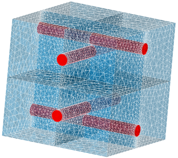
Figure 10.3-a : mesh e of the plate section for identifying the parameters of DHRC
The mesh presented at, obtained with the identification tool [SU1.10.01], thus represents a section of the studied plate of \(10\times 10\times 10{\mathit{cm}}^{3}\) with steels of diameter \(10\mathit{mm}\) corresponding to a reinforcement rate for each reinforcement sheet of \(8.0\times {10}^{-4}{m}^{2}/m\).
The properties of the materials selected for identification are summarized in the table below:
\({E}_{a}\), \(\mathrm{MPa}\) |
|
|
, |
|
|
|
|
|
, |
, |
, |
, |
, \({\sigma }_{d}\) \(\mathrm{MPa}\) \({\tau }_{\mathrm{crit}}\) \(\mathrm{MPa}\) |
|||
200,000 |
0.2 |
32,308 |
32,308 |
0.2 |
0.2 |
0.8 |
1.7 |
1.7 |
1.6 |
10.3.2. Characteristics of modeling#
Apart from the parameters, modeling with model DHRCrepose on the same mesh and the same characteristics as that with model GLRC_DM.
10.4. Tested values and results#
The average reaction forces along the axis \(\mathit{Ox}\) and the average displacements along the axis \(\mathit{Oy}\) en \(\mathrm{A2}-\mathrm{A4}\) obtained by multi-layer modeling (reference) and by the models based on the models GLRC_DMetDHRC are compared, in terms of relative differences; the tolerance is taken as an absolute value on these relative differences; the tolerance is taken as an absolute value on these relative differences:
Identification |
Reference type |
Reference value |
Tolerance |
TRACTION - ELASTIQUE \(t=\mathrm{0,25}\) |
|||
Relative difference \(\mathit{FX}\) EIB - GLRC_DM |
|
0.26455822871111 |
1 10-6 |
Relative difference \(\mathrm{DY}\) EIB - GLRC_DM |
|
0.57056458807998 |
1 10-6 |
TRACTION - ENDOMMAGEMENT \(t=\mathrm{1,0}\) |
|||
Relative difference \(\mathrm{FX}\) EIB - GLRC_DM |
|
0.81484181214706 |
1 10-6 |
TRACTION - DECHARGEMENT \(t=\mathrm{1,5}\) |
|||
Relative difference \(\mathrm{FX}\) EIB - GLRC_DM |
|
0.81484181214706 |
1 10-6 |
COMPRESSION - CHARGEMENT \(t=\mathrm{2,5}\) |
|||
Relative difference \(\mathrm{FX}\) EIB - GLRC_DM |
|
-0.093933297095696 |
1 10-6 |
COMPRESSION - DECHARGEMENT \(t=\mathrm{3,5}\) |
|||
Relative difference \(\mathrm{FX}\) EIB - GLRC_DM |
|
-0.093933297003640 |
1 10-6 |
Identification |
Reference type |
Reference value |
Tolerance |
TRACTION - ELASTIQUE \(t=\mathrm{0,05}\) |
|||
Relative difference \(\mathit{FX}\) DHRC - GLRC_DM |
|
-6.60608828608E-08 |
1 10-6 |
Relative difference \(\mathit{DY}\) DHRC - GLRC_DM |
|
-0.0688279909399 |
1 10-6 |
TRACTION - ENDOMMAGEMENT \(t=\mathrm{0,25}\) |
|||
Relative difference \(\mathit{FX}\) DHRC - GLRC_DM |
|
0.0785537404869 |
1 10-6 |
Relative difference \(\mathit{DY}\) DHRC - GLRC_DM |
|
-0.398169320815 |
1 10-6 |
TRACTION - GLISSEMENT \(t=\mathrm{0,8}\) |
|||
Relative difference \(\mathit{FX}\) DHRC - GLRC_DM |
|
0.0416150757582 |
1 10-6 |
Relative difference \(\mathit{DY}\) DHRC - GLRC_DM |
|
-0.680937900911 |
1 10-6 |
TRACTION - DECHARGEMENT \(t=\mathrm{1,5}\) |
|||
Relative difference \(\mathit{FX}\) DHRC - GLRC_DM |
|
0.0287804469267 |
1 10-6 |
Relative difference \(\mathit{DY}\) DHRC - GLRC_DM |
|
-0.71322832543 |
1 10-6 |
COMPRESSION - CHARGEMENT \(t=\mathrm{2,5}\) |
|||
Relative difference \(\mathit{FX}\) DHRC - GLRC_DM |
|
0.00314213260327 |
1 10-6 |
Relative difference \(\mathit{DY}\) DHRC - GLRC_DM |
|
-0.322634293852 |
1 10-6 |
COMPRESSION - DECHARGEMENT \(t=\mathrm{3,5}\) |
|||
Relative difference \(\mathit{FX}\) DHRC - GLRC_DM |
|
0.0245224165386 |
1 10-6 |
Relative difference \(\mathit{DY}\) DHRC - GLRC_DM |
|
-0.355143926407 |
1 10-6 |
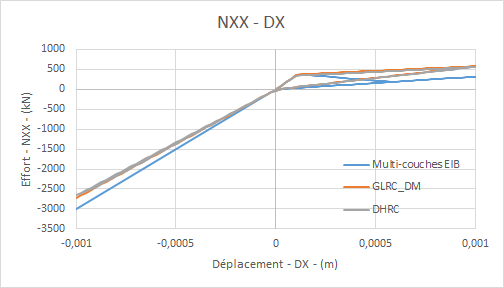
Comparative effort graphs \({N}_{\mathrm{xx}}\) — displacement \(\mathrm{DX}\) in traction/compression for load \(f\) :: **
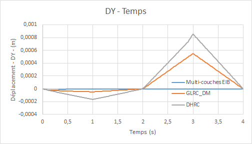
Comparative graphs displacement \(\mathrm{DY}\) (due to the Poisson effect) as a function of time:
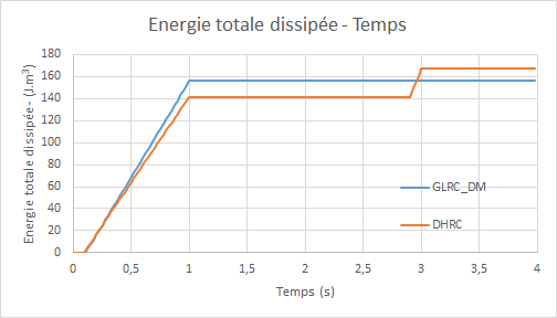
Diagrams of the evolution of the total energy dissipated by the models **** GLRC_DM and DHRC **** as a function of time:
10.5. notes#
The test case carried out here aims to test models GLRC_DM and DHRC under loads that are significant enough for the stiffness of the steels to effectively recover on the reference EIB. This test case uses test case SSNS106A by adding the reference DHRC in order to compare the global model GLRC_DM with a model taking into account more energy dissipation via the representation of sliding mechanisms internal to the steel-concrete interface. We notice on the Force-Displacement curve that the answer given by DHRC seems identical to that of GLRC_DM since there is no activation of sliding between the steels and the concrete.
On the other hand, on the curve of displacements \(\mathrm{DY}\) due to the Poisson effect, we notice large differences between the curves of the GLRC_DMet DHRC models and the curve of the model EIB. This is explained by the fact that the movements \(\mathrm{DY}\) are calculated, in the multi-layer calculation (EIB) on the layers of concrete, but the stress applied is such that the concrete reaches its tensile strength limit around the moment \(0.1s\).