3. Modeling A#
3.1. Characteristics of modeling#
Traction - compression - pure traction.
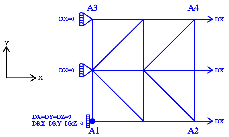
Figure 3.1-a: mesh and boundary conditions.
Modeling: DKTG
Boundary conditions:
Embedding in \({A}_{1}\);
\(\mathrm{DX}=0.0\) on the \({A}_{1}-{A}_{3}\) edge;
\(\mathrm{DX}={U}_{0}\times f(t)\) on the \({A}_{2}-{A}_{4}\) edge;
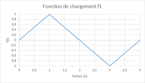
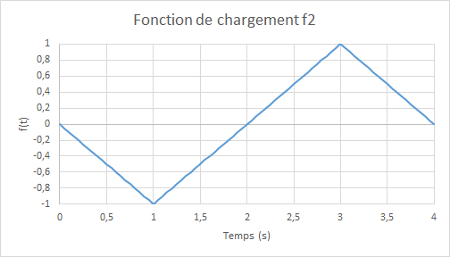
where \({U}_{0}=2.0\times {10}^{-4}m\) and \(f(t)\) represent the amplitude of cyclic loading as a function of the (pseudo-time) parameter \(t\). To properly verify the model, two loading functions are considered as follows:
|
|
Figure 3.1-b: Load functions f1 (left) and f2 (right).
Note: the extreme deformation is: \(2.0\times {10}^{-4}\) , which is well below the transition to plasticity of steels. No integration time: \(0.05s\) .
3.2. Characteristics of the mesh#
Number of knots: 9. Number of stitches: 8 TRIA3; 8 SEG2.
3.3. Tested values and results for the f1 loading function#
The average reaction forces along the axis \(\mathrm{Ox}\) and the average displacements along the axis \(\mathrm{Oy}\) and \(\mathrm{A2}-\mathrm{A4}\) obtained by multi-layer modeling (reference) and by that based on the model GLRC_DM are compared, in terms of relative differences; the tolerance is taken as an absolute value on these relative differences; the tolerance is taken as an absolute value on these relative differences:
Identification |
Reference type |
Reference value |
Tolerance |
|
TRAC. - PHASE CHAR. ELAS. \(t=\mathrm{0,25}\) |
||||
Relative difference in efforts \({N}_{\mathrm{xx}}\) |
|
0 |
5 10-2 |
|
Relative difference in displacement \(\mathrm{DY}\) |
|
0 |
5 10-2 |
|
TRAC. - PHASE CHAR. ENDO. \(t=\mathrm{1,0}\) |
||||
Relative difference in efforts \({N}_{\mathrm{xx}}\) |
|
0 |
1.2 10-1 |
|
Relative difference in displacement \(\mathrm{DY}\) |
|
0 |
1.7 10-1 |
|
TRAC. - PHASE DECHAR. ELAS. \(t=\mathrm{1,5}\) |
||||
Relative difference in efforts \({N}_{\mathrm{xx}}\) |
|
0 |
1.2 10-1 |
|
Relative difference in displacement \(\mathrm{DY}\) |
|
0 |
1.7 10-1 |
|
COMPR. - PHASE CHAR. ELAS. \(t=\mathrm{3,0}\) |
||||
Relative difference in efforts \({N}_{\mathrm{xx}}\) |
|
0 |
5 10-2 |
|
Relative difference in displacement \(\mathrm{DY}\) |
|
0 |
1.7 10-1 |
|
COMPR. - PHASE DECHAR. ELAS \(t=\mathrm{3,5}\) |
||||
Relative difference in efforts \({N}_{\mathrm{xx}}\) |
|
0 |
5 10-2 |
|
Relative difference in displacement \(\mathrm{DY}\) |
|
0 |
1.7 10-1 |
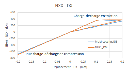
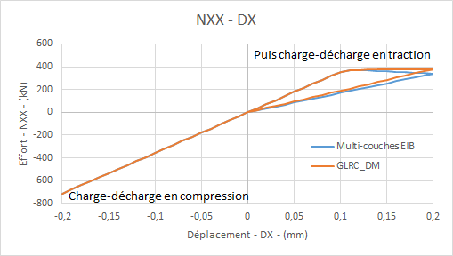
Comparative graphs efforts \({N}_{\mathrm{xx}}\) — displacement \(\mathrm{DX}\) in traction/compression for load \(\mathrm{f1}\) :: **
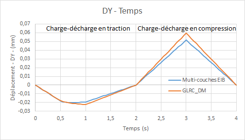
Comparative graphs displacement \(\mathrm{DY}\) (due to the Poisson effect) as a function of time:
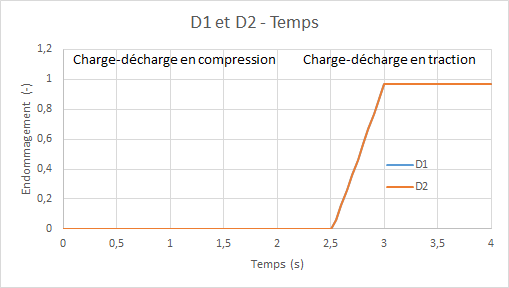
Diagrams of the evolution of the damage of model GLRC_DM (\({d}_{1}\) for the upper side and \({d}_{2}\) for the lower side) as a function of time:
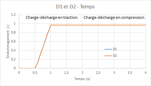
Using the damage variables, we also test the energy dissipated, which is written as: [R7.01.32 §2.7]:
\(E\mathrm{=}{k}_{0}\mathrm{\times }({d}_{1}+{d}_{2})\) with here \({k}_{0}\mathrm{=}8.89910J\mathrm{/}{m}^{2}\)
The energy dissipated therefore has the same profile as the curve above.
3.4. Tested values and results for the f2 loading function#
The average reaction forces along the axis \(\mathrm{Ox}\) and the average displacements along the axis \(\mathrm{Oy}\) and \(\mathrm{A2}-\mathrm{A4}\) obtained by multi-layer modeling (reference) and by that based on the model GLRC_DM are compared, in terms of relative differences; the tolerance is taken as an absolute value for these relative differences; the tolerance is taken as an absolute value for these relative differences:
Identification |
Reference type |
Reference value |
tolerance |
|
COMPR. - PHASE CHAR. ELAS. \(t=\mathrm{0,25}\) |
||||
Relative difference in efforts \({N}_{\mathit{xx}}\) |
|
0 |
5 10-2 |
|
Relative difference in displacement \(\mathrm{DY}\) |
|
0 |
5 10-2 |
|
COMPR, - PHASE CHAR. ENDO. \(t=\mathrm{1,0}\) |
||||
Relative difference in efforts \({N}_{\mathrm{xx}}\) |
|
0 |
5 10-2 |
|
Relative difference in displacement \(\mathrm{DY}\) |
|
0 |
5 10-2 |
|
COMPR. - PHASE DECHAR. ELAS. \(t=\mathrm{1,5}\) |
||||
Relative difference in efforts \({N}_{\mathrm{xx}}\) |
|
0 |
5 10-2 |
|
Relative difference in displacement \(\mathrm{DY}\) |
|
0 |
5 10-2 |
|
TRAC. - PHASE CHAR. ELAS. \(t=\mathrm{3,0}\) |
||||
Relative difference in efforts \({N}_{\mathrm{xx}}\) |
|
0 |
1.2 10-1 |
|
Relative difference in displacement \(\mathrm{DY}\) |
|
0 |
1.7 10-1 |
|
TRAC. - PHASE DECHAR. ELAS. \(t=\mathrm{3,5}\) |
||||
Relative difference in efforts \({N}_{\mathrm{xx}}\) |
|
0 |
1.2 10-1 |
|
Relative difference in displacement \(\mathrm{DY}\) |
|
0 |
1.7 10-1 |
Comparative graphs \({N}_{\mathrm{xx}}\) — displacement \(\mathrm{DX}\) in traction/compression for load \(\mathrm{f2}\) :: **
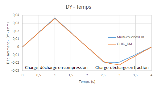
Comparative graphs displacement \(\mathrm{DY}\) (due to the Poisson effect) as a function of time:
Diagrams of the evolution of the damage of model GLRC_DM (\({d}_{1}\) for the upper side and \({d}_{2}\) for the lower side) as a function of time:
3.5. notes#
According to the preceding curves, it can be seen that model GLRC_DM represents the overall behavior of reinforced concrete under tensile — pure compression in a satisfactory manner. The relative error of model GLRC_DM with respect to the reference solution is admissible. It should be noted that the difference between model GLRC_DM and ENDO_ISOT_BETON is the most important during the damage phase: the behavior of concrete under tension is then softening and we find a negative slope in the multi-layer reference model, despite the reinforcement (steel layers and layers ENDO_ISOT_BETON) while one of the hypotheses of the model GLRC_DM is not to model the softening of reinforced concrete.
Being based on the isotropic equivalent material hypothesis (see [R7.01.32]), the GLRC_DM model slightly overestimates the Poisson effect.
We also check the symmetry of the response according to the chosen direction of compression-traction load or the opposite, depending on the load \(\mathit{f1}\) or \(\mathit{f2}\).