6. D modeling#
6.1. Characteristics of modeling#
Pure in-plane distortion and shear.
|
|
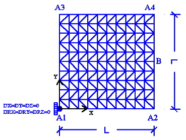
Figure 6.1-a: Meshing and boundary conditions.
Modeling: DKTG. \(L=1.0m\).
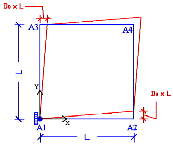
Boundary conditions (see figure above on the right) so that the plate is subject to pure distortion: \({\varepsilon }_{\text{xy}}\) must be constant or to pure shear: forces are applied. Therefore, the following displacement field is applied to the edges of the plate for distortion:
\(\mathrm{\{}\begin{array}{c}{u}_{x}\mathrm{=}{D}_{0}\mathrm{\cdot }y\\ {u}_{y}\mathrm{=}{D}_{0}\mathrm{\cdot }x\end{array}\mathrm{\Rightarrow }\varepsilon \mathrm{=}\frac{1}{2}({u}_{x,y}+{u}_{y,x})\mathrm{=}{D}_{0}\)
So:
we impose an embedding in \({A}_{1}\),
\({u}_{x}={D}_{0}\cdot y,{u}_{y}=0\) on edge \({A}_{1}-{A}_{3}\), \({u}_{x}=0,{u}_{y}={D}_{0}\cdot x\) on edge \({A}_{1}-{A}_{2}\),
\({u}_{x}={D}_{0}\cdot y,{u}_{y}={D}_{0}\cdot L\) on edge \({A}_{2}-{A}_{4}\), \({u}_{x}={D}_{0}\cdot L,{u}_{y}={D}_{0}\cdot x\) on edge \({A}_{3}-{A}_{4}\),
where \({D}_{0}=3.3{10}^{-4}\) and \(f(t)\) represent the magnitude of cyclic loading as a function of the (pseudo-time) parameter \(t\), defined as:
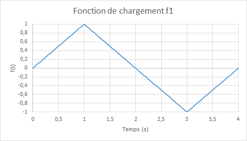
Figure 6.1-b: loading function
Integration increment: \(0.05s\).
For shearing, the following forces are applied:
we impose \({F}_{y}={D}_{0}\) on \({A}_{2}{A}_{4}\),
we impose \({F}_{x}={D}_{0}\) on \({A}_{4}{A}_{3}\),
we impose \({F}_{y}=-{D}_{0}\) on \({A}_{3}{A}_{1}\),
we impose \({F}_{x}=-{D}_{0}\) on \({A}_{1}{A}_{2}\),
6.2. Characteristics of the mesh#
Knots: 121.
Stitches: 200 TRIA3; 40 SEG2.
6.3. Tested sizes and results#
For the distortion, the shear force \({N}_{\mathrm{xy}}\) and \(B\) obtained by the two models are compared; the tolerances are taken in absolute values based on these relative differences:
Identification |
Reference type |
Reference value |
Tolerance |
|
DIST. POS. - PHASE CHAR. ELAS. \(t=\mathrm{0,25}\) |
||||
Relative difference in efforts \({N}_{\mathrm{xy}}\) |
|
0 |
5 10-2 |
|
DIST. POS. - PHASE CHAR. ENDO. \(t=\mathrm{1,0}\) |
||||
Relative difference in efforts \({N}_{\mathrm{xy}}\) |
|
0 |
7 10 -2 |
|
DIST. POS. - PHASE DECHAR. ELAS. \(t=\mathrm{1,5}\) |
||||
Relative difference in efforts \({N}_{\mathrm{xy}}\) |
|
0 |
7 10 -2 |
|
DIST. NEG. - PHASE CHAR. ELAS. \(t=\mathrm{3,0}\) |
||||
Relative difference in efforts \({N}_{\mathrm{xy}}\) |
|
0 |
7 10-2 |
|
DIST. NEG. - PHASE DECHAR. ELAS. \(t=\mathrm{3,5}\) |
||||
Relative difference in efforts \({N}_{\mathrm{xy}}\) |
|
0 |
7 10-2 |
Shearing force diagram \({N}_{\mathrm{xy}}\) (in the plan) as a function of time:
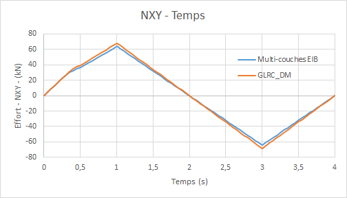
shear force graph \({N}_{\mathit{xy}}\) **** (in the plan) **based on:math:`{D}_{0}`**imposed: **
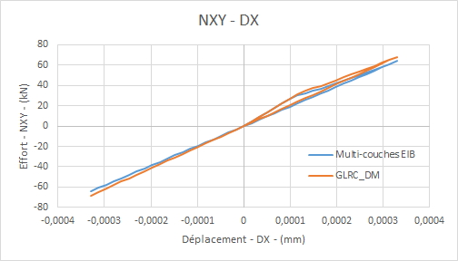
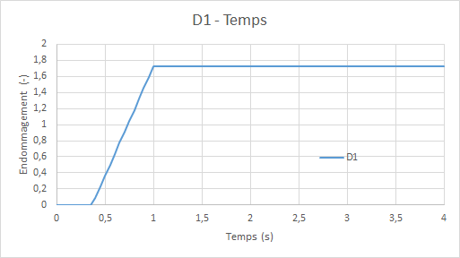
Diagram of the evolution of model damage **** GLRC_DM **** ( \({d}_{1}={d}_{2}\) ) as a function of time:
For shear, we do non-regression tests on shear deformations \({\varepsilon }_{\mathrm{xy}}\) in \(B\):
Identification |
Reference type |
Reference value |
Tolerance |
|
CIS. POS. - PHASE CHAR. ELAS. \(t=\mathrm{0,1}\) |
||||
Shear Deformations \({\varepsilon }_{\mathrm{xy}}\) |
|
3.013 10-15 |
1 10-6 |
|
CIS. POS. - PHASE CHAR. ENDO. \(t=\mathrm{0,8}\) |
||||
Shear deformations \({\varepsilon }_{\mathrm{xy}}\) |
|
2,410 10-14 |
7 10 -2 |
6.4. notes#
In order to have a better agreement between model GLRC_DM and the reference (multilayer model) in pure distortion, it was necessary to modify the Young’s modulus from \(E=35620\mathit{MPa}\) to \(E=42500\mathit{MPa}\) compared to the A, B, C models, knowing that in pure distortion the steels are not loaded.
It is verified that the shear force obtained with Code_Aster at time \(t=\mathrm{0,37427}s\), just when the first damage occurs, produces the theoretical elastic value:
\({N}_{\mathrm{xy}}^{D}=2\frac{\sqrt{2{\mu }_{m}{k}_{0}}}{\sqrt{2-{\gamma }_{\mathrm{mc}}-{\gamma }_{\mathrm{mt}}}}=\frac{{N}_{D}}{1+{\nu }_{m}}\cdot \sqrt{\frac{(1-{\nu }_{m})(1+2{\nu }_{m})(1-{\gamma }_{\mathrm{mt}})+{\nu }_{m}^{2}(1-{\gamma }_{\mathrm{mc}})}{2-{\gamma }_{\mathrm{mc}}-{\gamma }_{\mathrm{mt}}}}\)
that is: \({N}_{\mathrm{xy}}^{D}=331128N/m\).