8. G modeling — non-linear dynamics with substructuring

8.1. Objective

This TP follows the modeling E (non-linear dynamics). The objective of this TP is to set up a transient non-linear calculation with DYNA_NON_LINE taking into account dynamic substructuring.

Dynamic substructuring consists in partitioning the structure into one or more substructures in order to reduce the size of the numerical model and to be able to study each substructure independently. The overall model is then obtained by assembling the models of the various substructures.

Each substructure is projected onto a carefully selected vector base. This projection makes it possible to reduce the size of the model of each substructure and therefore the size of the model of the assembled structure.

The behavior of the substructure must be linear. The portion of the plate in which the non-linear behavior (plasticity) was observed in the E model will remain represented in the physical base. The choice of the region of the model to apply the substructuring method must therefore be made wisely.

The following figure shows the elements that have plasticized (in red) along the transient of modeling E, which corresponds to the region close to the embedment of the plate:

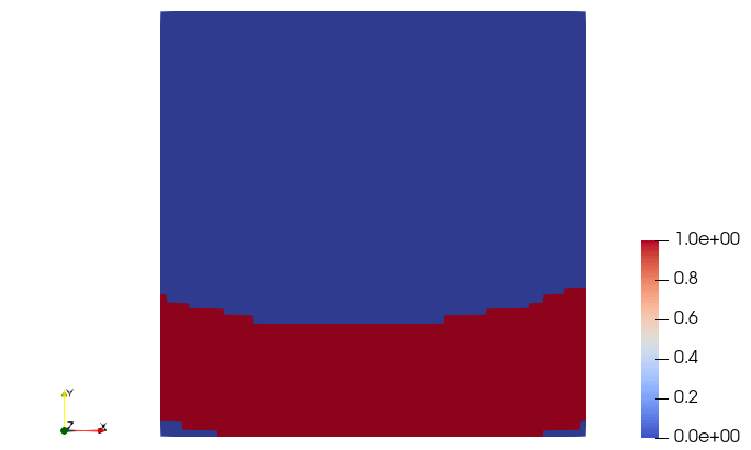
Fig. 8.1 Result of modeling E with the plasticized area in red.

Half of the model remaining linear (side opposite to embedding) will therefore be subject to the substructuring procedure:

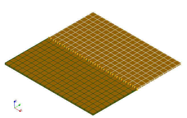
Fig. 8.2 Meshing with two GROUP_MA for substructuring

To carry out this study, the forma12g.med mesh was enriched with the creation of a group of elements (VOL_1) representing the part that will be modeled on a physical basis (embedded side), a group of elements (VOL_2) representing the part that will be represented in a reduced base, and a group of nodes (No_Int) at the interface of these two areas of the model.

8.2. Calculation procedure

8.2.1. Creation of the dynamic macro element

The first step is to create the dynamic macro element that will represent the behavior of the condensed part of the structure in the final model. For this, the Craig-Bampton method will be applied. This step is only done on the mesh’s VOL_2 element group.

The Craig-Bampton technique consists in choosing normal modes and constrained modes as the basis for projection. Normal modes are modes specific to the substructure where all the nodes of the interfaces with the adjacent substructures are blocked. A constrained mode is defined by the static deformation obtained by imposing a unit displacement on one degree of freedom of connection, the other degrees of freedom of connection being blocked. The projection base contains normal modes and all the all the constrained modes associated with all the degrees of bond freedom.

To calculate the normal modes, we must therefore embed the group of nodes of the No_Int interface with the AFFE_CHAR_MECA operator. Before assembling the mass and stiffness matrices necessary for the calculation of normal modes, we take the opportunity to create the load applied to the VOL_2 group, which will also compose the dynamic macro-element. We then execute the ASSEMBLAGE operator with the options RIGI_MECA, * , MASS_MECA , AMOR_MECA , and CHAR_MECA.

We calculate the normal modes with CALC_MODES. Attention, the number of modes selected must be a multiple of the number of DDL of the finite elements that make up the condensed domain (3 in this case), keyword CALC_FREQ =_F (NMAX_FREQ =30).

Constrained modes are calculated with the MODE_STATIQUE operator, keywords MODE_STAT =( _F (GROUP_NO = »No_Int », AVEC_CMP =( « DX », « DY », « DZ »)))).

Then we must define the dynamic interface with DEFI_INTERF_DYNA, keyword TYPE =” =” CRAIGB “, in order to be able to define the modal base containing the normal modes, the constrained modes and the dynamic interface using the DEFI_BASE_MODALE operator.

We get the numbering of the new database using NUME_DDL_GENE , and we project the load on this base with PROJ_VECT_BASE *.

The macro element is constructed by the MACR_ELEM_DYNA operator with the keywords BASE_MODALE and CAS_CHARGE. We then use DEFI_MAILLAGE with the keyword DEFI_SUPER_MAILLE to define a new mesh based on the dynamic macro element. This new mesh must then be assembled to the TP base mesh, forma12g.med, using the ASSE_MAILLAGE * operator.

8.2.2. Model construction

Once the macro-element has been generated and integrated into the initial mesh, the second step of this TP consists in building the plate model, which will have one half represented in the physical base, and the other by the dynamic macro-element. The macro-element is taken into account in the model using the keyword AFFE_SOUS_STRUC and the operator AFFE_MODELE *.

Once the elasto-plastic material has been assigned to the group of physical elements” VOL_1 “and the embedment boundary conditions have been applied to the edge of the plate, it is important, as a check, to calculate the natural modes of the model, to verify whether the macro-element has been properly constructed and integrated into the model that will be used later.

The rest of the calculation takes place as in modeling E, the only difference being that in the DYNA_NON_LINE operator, the keyword SOUS_STRUC must be added with the argument CAS_CHARGE so that the load applied to the part of the model that has been condensed is taken into account.

Once the calculation is complete, the REST_COND_TRAN operator allows you to retrieve the fields in the condensed part of the model. The rest of the post-processing takes place in the same way as the E modeling.

8.3. Results

The following figures show the displacement, speed, and acceleration at point P of the model, for E (full model) and G (with dynamic substructuring) models. It is observed that the curves are superimposed.

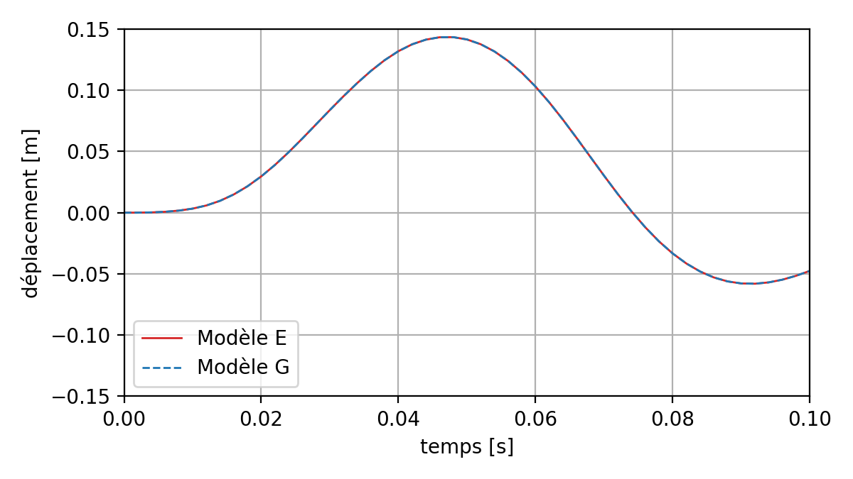
Fig. 8.3 Comparison of the displacements at point P between two direct and substructured nonlinear transient calculations

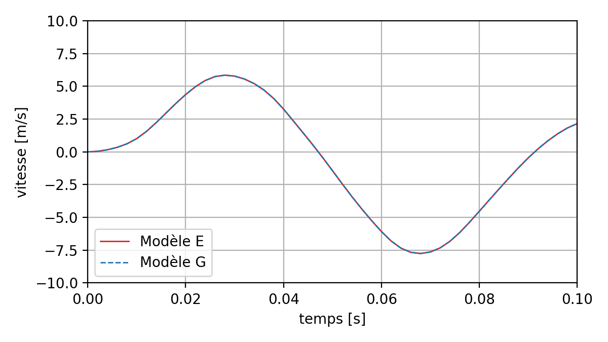
Fig. 8.4 Comparison of velocities at point P between two nonlinear transient calculations (direct and by substructuring)

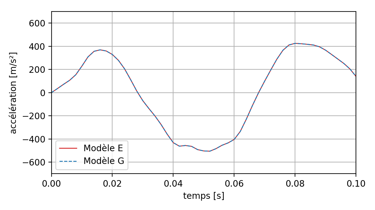
Fig. 8.5 Comparison of accelerations at point P between two nonlinear transient calculations (direct and by substructuring)