4. C modeling — transient analysis on a modal basis#
4.1. Problem and clues#
Transitional analysis can also be done more effectively by projecting the problem on a modal basis. It is proposed to compare this method with the direct transitory calculation.
First, it is proposed to solve the transient on the family of modes determined in the modeling A. To do this, a modal base is constructed with the previous modes, the matrices and the vectors are projected into this new base and the transient is solved. These steps are specified below:
calculation of modes as in modeling A
construction of a vector containing the second member by* CALC_VECT_ELEM and ASSE_VECTEUR *
definition of a modal base by* DEFI_BASE_MODALE *
creation of a generalized numbering by* NUME_DDL_GENE *
If the base is orthonormal, it can be indicated by the keyword* STOCKAGE =” DIAG “*
projection of mass, stiffness, and load vector matrices:* PROJ_VECT_BASE and PROJ_MATR_BASE *
as the vector is a loading, we indicate* TYPE_VECT =” FORC “*
transitory calculation on a modal basis:* DYNA_VIBRA (TYPE_CALCUL =” TRANS “, BASE_CALCUL =” GENE”) *
we calculate the answer up to \(0.5s\) with a time step of \(0.002s\)
recovery of the movement of point P by* RECU_FONCTION (RESU_GENE) *
It is appropriate to ask ourselves on what basis this displacement is expressed then
printing of the displacement/time curve:* IMPR_FONCTION *
It should be noted that the DYNA_LINE command provides all these steps in a very synthetic way. Attention: by default, this command determines static enrichment. To not do this, you must specify ENRI_STAT =” NON “.
4.2. Results of calculations on a modal basis without static correction#
For vertical displacement, results are obtained that are very similar to the direct transitory calculation.
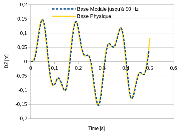
Fig. 4.1 Comparison of movements in DZ at point P between physical and modal bases up to 50 Hz#
But if you look at the movements in the horizontal direction, they are quite different!!!
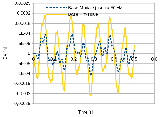
Fig. 4.2 Comparison of DX movements at point P between physical and modal bases up to 50 Hz#
Although the modal base was calculated beyond \(50\mathit{Hz}\) and the usual rule was respected, recommending to cover twice the maximum frequency of the excitation, in the horizontal direction, the modal projection method is far from the direct result.
What happened?
The plate is in fact very steep in its plane (horizontal direction). The specific modes therefore represent this movement only imperfectly. To reproduce it correctly, you would have to use many more modes of its own.
4.3. Calculations on a modal basis with static correction a priory#
However, one method is much more efficient. This is the static correction method, which makes it possible to take into account the « static » contribution of the structure to the movement. It can be done in 2 ways:
a priory: a new mode is integrated into the modal base on which to solve the transient;
a posteriori: the initial modal base is retained but a correction is added to the solution obtained.
We are going to look at these 2 possibilities.
First of all, static correction a priory (C modeling). The steps of the transient calculation on a modal basis with a priory static correction are as follows:
Plate modes up to 50 Hz are calculated via* CALC_MODES *.
Pseudo-mode is calculated via* MODE_STATIQUE/SPEUDO_MODE *.
A new modal base is defined by adding static mode to « dynamic » modes by* DEFI_BASE_MODALE/RITZ *.
As these different modes are a principle not orthogonal to each other, we specify* ORTHO =” OUI “* to perform orthonormalization. We must also indicate which matrix will be used for this operation (orthogonality in the matrix norm).
Creation of a generalized numbering by* NUME_DDL_GENE *
If the base is orthonormal, it can be indicated by the keyword* STOCKAGE =” DIAG “*
projection of mass, stiffness, and load vector matrices:* PROJ_VECT_BASE and PROJ_MATR_BASE *
As the vector is a loading, we indicate* TYPE_VECT =” FORC “*
Transitional calculation on a modal basis:* DYNA_VIBRA (TYPE_CALCUL =” TRANS “, BASE_CALCUL =” GENE”) *
We calculate the answer up to \(0.5s\) with a time step of \(0.002s\)
We use the Devogelaere-Fu time scheme by* SCHEMA_TEMPS/SCHEMA =” DEVOGE “*
construction of the overall response of the structure on a physical basis by* REST_GENE_PHYS *
recovering the movement of the point P* RECU_FONCTION (RESULTAT) *
printing of the displacement/time curve:* IMPR_FONCTION *
It should be noted that the DYNA_LINE command provides all these steps in a very synthetic way.
The static correction a posteriori will be treated in the D modeling.
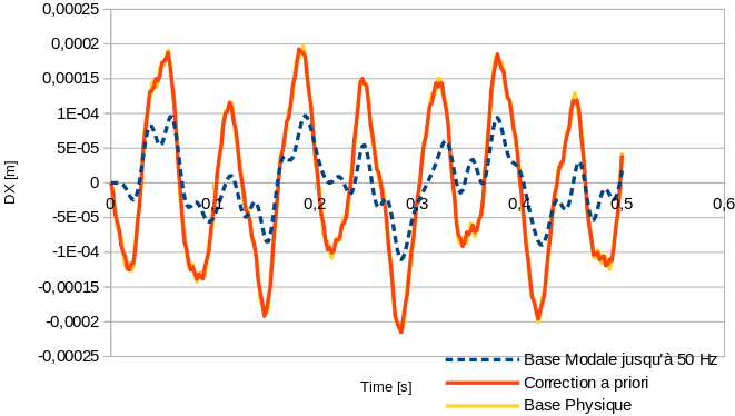
Fig. 4.3 Comparison of DX movements at point P between physical and modal bases up to 50 Hz with prior correction#
4.4. Taking depreciation into account in calculations on a modal basis with static correction a priory#
It is proposed to take depreciation into account in the context of the calculations carried out previously. With this in mind, damping is here modelled via a reduced damping coefficient, equal to:math: xi =1.86%.
For each case (i.e., modal basis, static correction a priory, DYNA_LINE, ), we proceed in a purely analogous manner to calculations without damping, by specifying the abovementioned reduced damping coefficient via the keywords AMOR_MODAL/AMOR_REDUIT in the case of the/* ** * ** in the case of the * ** * ** in the case of the operator DYNA_VIBRA , and via the keyword , and via the keyword AMORTISSEMENT in the case of the operator DYNA_LINE *.
The temporal evolution of the DZ component of the displacements obtained with and without damping, in the case of a transient calculation on a modal basis with a prior static correction is presented below:
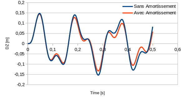
Fig. 4.4 Comparison of the movements in DX at point P between two calculations on a modal basis up to 50 Hz with prior correction, with and without modal damping at 1.86%#