5. Model D- static correction a posteriori#
5.1. Calculation procedure#
The steps are quite similar to the method without static correction. But a few steps are added to take into account the deformations due to the static effects of loading.
Careful! One should not forget to include the correction when returning to the physical base.
calculation of the modal base up to 50 Hz;
definition of gravity loading:
AFFE_CHAR_MECA (PESANTEUR =_F (GRAVITE =300. , DIRECTION =( -1,0.1))
static correction calculation:* MACRO_ELAST_MULT *
projection of mass, stiffness, and load vector matrices:* PROJ_BASE *
data of the multiplicative function in time (sine of period \(15\mathrm{\times }2\pi\) s):* FORMULE *
definition of a list of moments (You can take a list of moments on \(0.5s\) with a time step of \(0.002s\)):* DEFI_LIST_REEL *
We also need the first and second derivatives of the multiplicative time function: formula (if we know their analytic form or* CALC_FONCTION * for a numerical approximation)
transitory calculation on a modal basis:* DYNA_VIBRA (TYPE_CALCUL =” TRANS “, =””, BASE_CALCUL =” GENE “) — give behind MODE_CORR the static deformation and specify behind D_FONC_DT and D_FONC_DT2 * the first and second derivatives
recovering the movement of point P RECU_FONCTION (RESU_GENE) .Do not forget* CORR_STAT =” OUI “*
printing of the displacement/time curve:* IMPR_FONCTION *
5.2. Results#
Thanks to static correction afterwards, the results are much better.
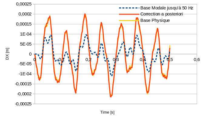
Fig. 5.1 Comparison of DX movements at point P between physical and modal bases with a posteriori static correction#