7. F modeling — linear dynamics with localized nonlinearities#
7.1. Objective#
This case is an introduction to using Code_Aster for dynamic transient analysis with localized nonlinearities. The shock behavior in question is of the elastic type. Nonlinearity is introduced by a displacement/speed/effort relationship at the nodes carrying the nonlinearities. The calculation is carried out using the Code_Aster linear dynamics operator DYNA_VIBRA. The resolution is based on an explicit integration diagram, non-linearity is treated with the second member of the equations of motion: * at time i, the displacements are calculated in order to achieve balance with the forces calculated at time i-1; * the forces at time i are calculated from the displacements thus calculated and they are applied at time i+1 in order to obtain the displacements at i+1. The response of the plate is calculated up to a final time of 1 second, and a normal shock stiffness equal to KN= 1E8N /m is considered.
7.2. Calculation framework#
A thick steel plate is deformed before it is dropped. Two contact points then limit the movement of the plate. The two contact points are arranged under the plate, facing each other from the ends of the free edge (Figure 7.1). When the plate is horizontal, there is no gap between the plate and the contact points. The geometry of the plate and the material are the same as those already used for the models a, b, c and d.
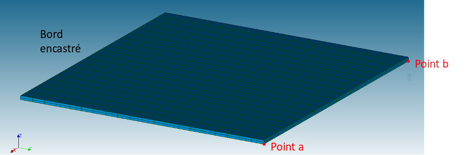
Fig. 7.1 Position of the shock points#
More precisely, the plate is pre-deformed by 0.25 m in the Z direction and then left free to vibrate. The contact will take place whenever, during the vibratory movement, the end nodes of the plate located on the lower surface return to their initial position before deformation.
7.3. Meshing#
The mesh of the plate is the same as that already used for the models a, b, c, d and e. However, it is necessary to create:
A group of CHOC_a2 and CHOC_b2 meshes that contain the end nodes of the plate positioned on the lower surface facing each other of the contact points;
LIBRE: it is a group of elements (* SEG2 *) at the free end of the plate, connecting node groups CHOC_a2 and CHOC_b2.
The static problem load assignment is done via the* MECA_STATIQUE * operator.
Boundary conditions and loading are imposed via the* EXCIT * keyword.
We then use the CREA_CHAMP command to create the displacement field which will then be the initial condition for the dynamic calculation. This is the displacement field calculated at the last moment of the static calculation. Attention, it is important to use, in the construction of the field, the same numbering of the degrees of freedom that was used during assembly, without the imposed displacement load.
7.4. Dynamic calculation#
Common steps include:
we calculate the modal base using the command* CALC_MODES *;
static modes are calculated using the* MODE_STATIQUE command. A unit force is imposed on the shock nodes b 2 and a 2 in order to calculate the static deformation of the plate under these conditions. The displacement field thus obtained is used to enrich the modal base of the plate in order to take into account its static response. Enrichment is done by the command DEFI_BASE_MODALE *;
the constructed base does not consist of orthogonal modes. It must then be orthogonalized. To do this we rely again on the command* DEFI_MODALE *;
we then project the mass and stiffness matrices onto the new base via the* PROJ_BASE * operator, but we must also project the displacement vector from the static calculation.
definition of the geometry of shock sites. The Aster command that allows you to define the geometry of the shock locations is* DEFI_OBSTACLE (user documentation U4.44.21). The key word TYPE makes it possible to define the physics of shock more precisely. For example, the keywords PLAN_Y , PLAN_Z , , ,, CERCLE, and DISCRET define the geometry of the contacts between a mobile structure and an undeformable obstacle. The types BI_PLAN_Y, BI_PLAN_Z, * , BI_CERCLE , and BI_CERC_INT allow you to define the possible places of contact between two mobile nodes. In the present case of a plate that comes into contact with fixed points in space, the type PLAN_Z * is chosen.
parameterization of the linear dynamics operator* DYNA_VIBRA (user documentation U4.53.03). The setting of DYNA_VIBRA * requires the definition of shock behavior. The keyword behavior must be present as many times as the number of touchpoints, so twice in this case. For each occurrence of the keyword behavior, you must then indicate:
what is the node group in the structure to which the behavior will be assigned (CHOC_a2 at the first occurrence of the behavior keyword, CHOC_b2 at the second)
whether the shock occurs with friction or not: keyword* FROTTEMENT *
the relationship of CHOC (* DIS_CHOC * for elastic contacts)
stiffness in the normal direction of impact:* RIGI_NORM *
the geometry of the place of impact;
normal to the direction of shock* NORM_OBST *;
the obstacle defined by the command* DEFI_OBSTACLE , keyword OBSTACLE *;
the origin of the obstacle via the keyword* ORIG_OBST *. This is the origin of the shock coordinate system;
normal to the direction of shock* NORM_OBST *;
the game, or the position of the shock plane in the shock coordinate system;
mass and stiffness matrices (those projected on the enriched and orthogonalized base)
the initial state (* ETAT_INIT *) including the static displacement projected on a modal basis
the integration diagram (we chose a Runge-Kutta type diagram, keyword* RUNGE_KUTTA_32 *), and the time increment (final moment and not. A step equal to 0.0001s was chosen for the study)
mass and stiffness matrices (those projected on the enriched and orthogonalized base)
In-fine: we report the results obtained on a physical basis using the REST_GENE_PHYS command. For this purpose, a time step of 0.001s is chosen. The definition of discretization in time for REST_GENE_PHYS is done via LIST_DEFI_REEL *.
We print the results in a .med file*via*using the* IMPR_RESU * command.
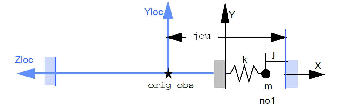
Fig. 7.2 Shock location geometry for elements PLAN_Z.#
RQ 1. Two shock planes that are symmetric with respect to the origin of the shock coordinate system are created automatically. In order to avoid contact of the structure with the plane that is not present in the modeling, it is advisable to move the origin of the coordinate system away from the obstacle of the structure. In the present case, it was chosen to position the origin of the coordinate system at a vertical distance of 1 m from the lower face of the plate. In this way the shock planes will be at the initial position, i.e. in contact with CHOC_a2 and CHOC_b2 before pre-deformation, (an example is shown in Figure 7.3-2 for point a), and the second shock plane will be far enough away from not coming into contact with CHOC_a2 and CHOC_b2 in the initial state.
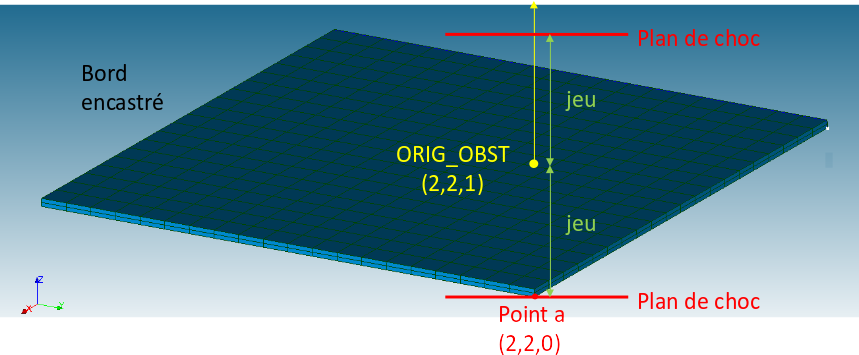
Fig. 7.3 Geometry of the place of shock in correspondence with point a.#
RQ 2. the choice of the integration step is a crucial element in terms of the quality of the solution when using explicit integration diagrams. A sufficiently refined time discretization must be chosen in order to obtain a converged solution. However, the resources mobilized by the calculation depend on time refinement. A study of sensitivity to temporal refinement is necessary in order to guide the choice.
7.5. Post-treatment and printing of results#
We recover the movements and the efforts over time in correspondence of the shock nodes using the RECU_FONCTION command.
The results at point b are printed in xmgrace format using the IMPR_RESU command.
Opening xmrgace files is done by command line via the command
xmgrage my file
Finally, remember that using the POST_DYNA_MODA_T command (Aster U4,84,02 documentation) (Aster U4,84,02 documentation), for each shock nonlinearity, we calculate and print in a table:
shock results and associated magnitudes:
For each shock, we have the value of the moment when the force is maximum, the value of the force
maximum and of the impulse, the duration of the shock, the speed of impact and the number of rebounds,
global shock data:
of all the shocks observed, we specify: the absolute maximum shock force, the
mean value of the maxima of shock forces and the standard deviation of the extremes of force of
Shocks
the histogram describing the maximum impact forces:
We have the number of classes in the histogram, the values of its abscissa (force, min and max)
of each class) and the probability density of the maximum strength of each class.
7.6. Questions#
Carry out the study taking into account only the vibratory mode of the plate and then gradually enrich the solution.
It should be noted that all the modes between 0 and 500 Hz affect the forces and movements at the point of contact and that, in addition, the use of an incomplete modal base can lead to error in the calculation of the shock force.
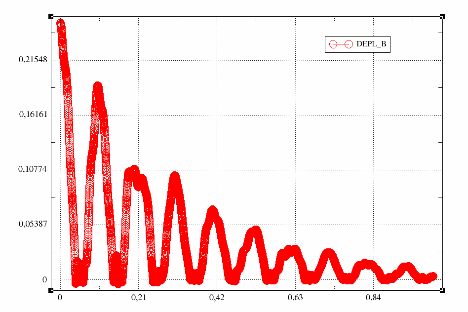
Fig. 7.4 Move to node b calculated with a single mode#
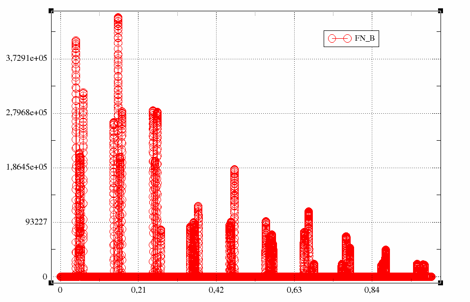
Fig. 7.5 Effort at node b calculated with a single mode#
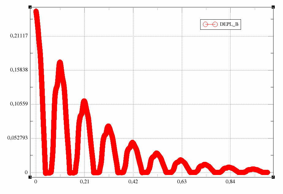
Fig. 7.6 Displacement at node b calculated with the natural modes calculated between 0 and 500 Hz#
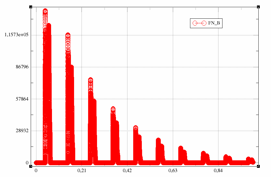
Fig. 7.7 Effort at node b calculated with natural modes calculated between 0 and 500 Hz#