2. Modeling A — Modal analysis

2.1. Objectives

To get an idea of the dynamic properties of the system, we start with a modal analysis.

The geometry is drawn and then meshed under Salome_Meca. The first modes of the plate are then calculated with Code_Aster.

2.1.1. Geometry in SALOME

The mesh is modelled in Salome.

In the Geometry module, we use the New Entity > Primitive > Box menu to build a box with the dimensions of the plate.

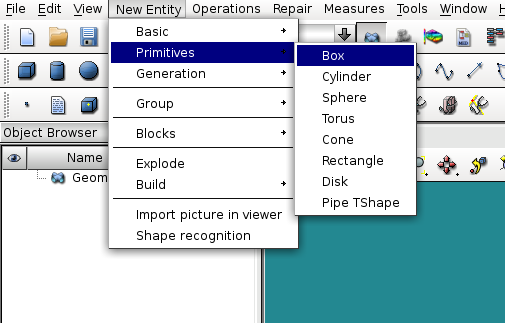
Fig. 2.1 Creating geometry via a box

To specify boundary conditions in Code_Aster and identify the nodes useful for post-processing, you need to name some geometry elements and some nodes.

It’s done thanks to*New Entity > Group > Create*.

The plate is fixed on one side. A point on the upper face, at an angle opposite to the embedded edge, is used as a post-processing node.

To be able to specify the fineness of the mesh in the thickness of the plate, it may be useful to create a group corresponding to the vertical edge of one of the corners of the plate.

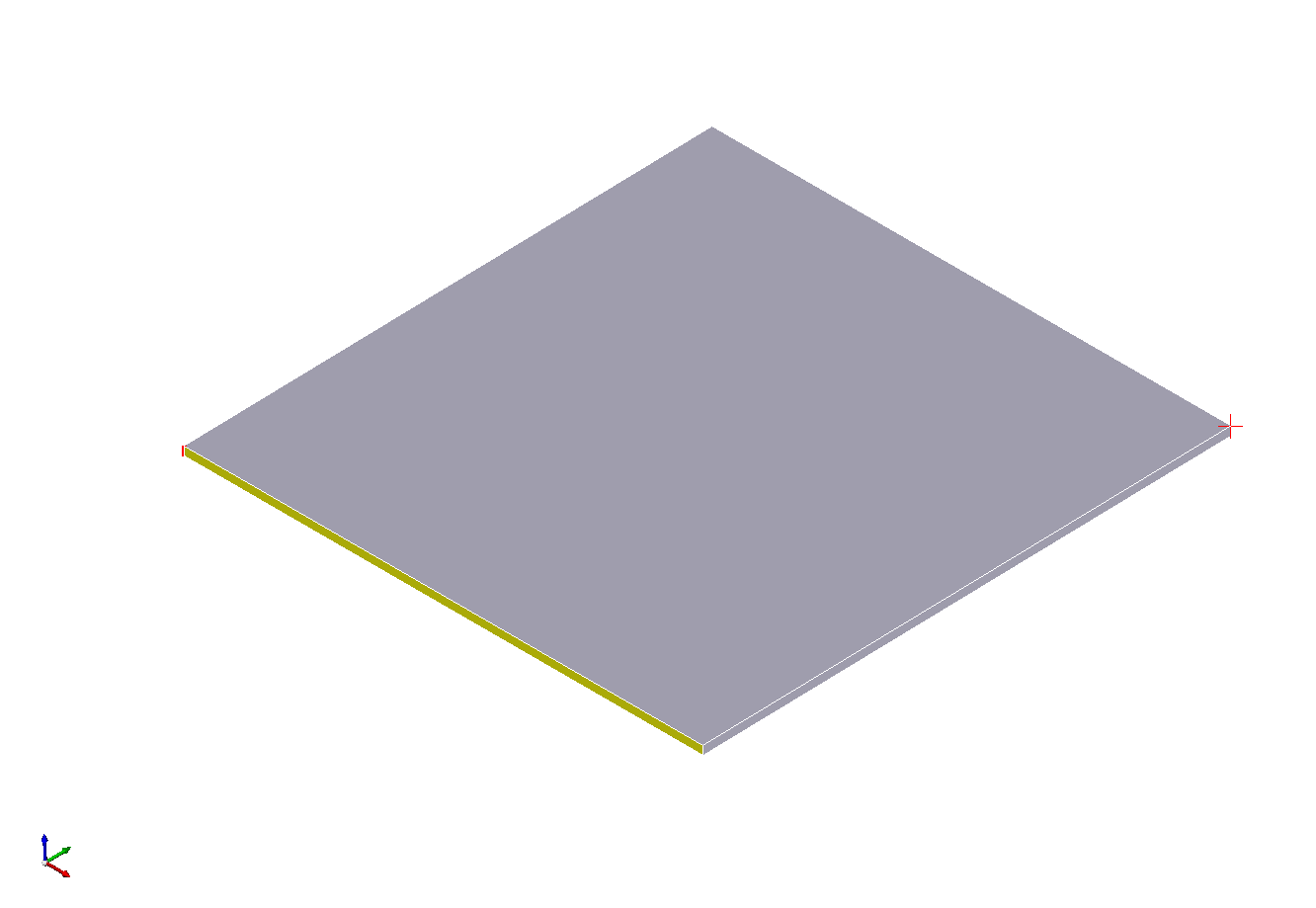
Fig. 2.2 Plate geometry

2.1.2. Meshing in SALOME

The next step is the creation of the mesh by the Mesh module. Numerous algorithms are available in the software.

To obtain a regulated and predictable mesh, one possible choice is:

Hexahedron (i, j, k) /Quadrangle (Mapping) /Wire discretisation, successively corresponding to 3D, 2D and 1D meshes.

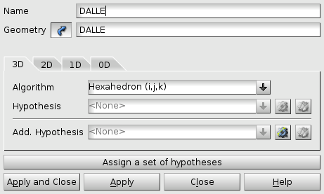
Fig. 2.3 Algorithm for generating the 3D mesh

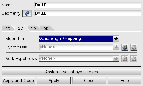
Fig. 2.4 Algorithm for generating the 2D mesh

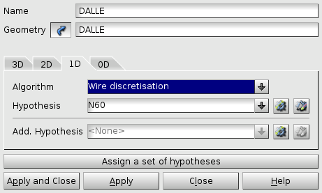
Fig. 2.5 Algorithm for generating the 1D mesh

To avoid a too fine mesh in the thickness of the plate, it is recommended to create a sub-mesh on one of the corner edges.

N.B.: do not forget to « spread » the discretization of the chosen corner edge to the others by specifying it in Add. Hypothesis.

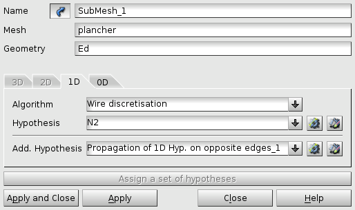
Fig. 2.6 Algorithm for generating the 1D mesh with the hypothesis of discretization of the edge

As a compromise between calculation time and precision, it is possible to create 40 elements in the width of the plate and 2 in the thickness.

A coarse mesh is then obtained but this defect can be compensated for by quadratic elements.

To switch from linear elements to quadratic elements we use the following option in the meshing menu: Modification > Convert to/from quadratic.

At the end of the procedure, the mesh includes 4725 nodes and 800 3D elements.

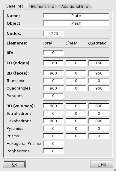
Fig. 2.7 Information about the mesh created

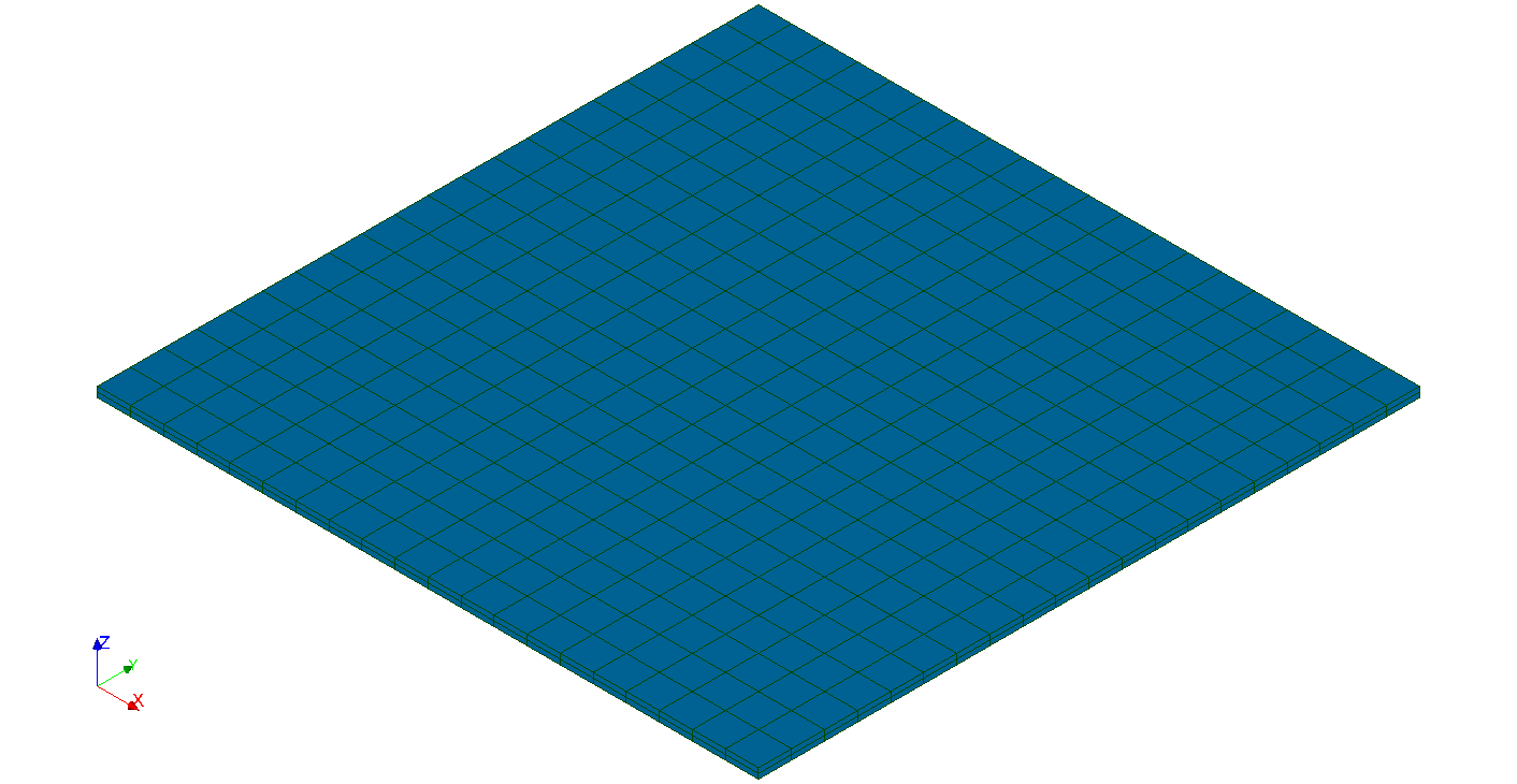
Fig. 2.8 Mesh created (3D view)

2.2. Modal analysis

First modes of the structure are required up to a frequency of \(50\mathit{Hz}\). This is a careful choice since the arousal frequency only amounts to \(15\mathit{Hz}\).

For this very simple calculation, the best solution is the use of an assistant. To do this, click « right paw » on the*Current case* entry in AsterStudy then on*Add Stage with Assistant*. Let yourself be guided and start your calculation in the History View tab.

Note that it may be necessary to increase the memory allocated to the calculation in the Memory box in the Run parameters window (see Fig. 2.9).

2.3. Post-treatment

For simple post-processing, it is very convenient to click « right paw » in the entry that corresponds to the file MEDde output in the Data Files Summary window (see Fig. 2.10).

You can browse the different modes by clicking on the button:

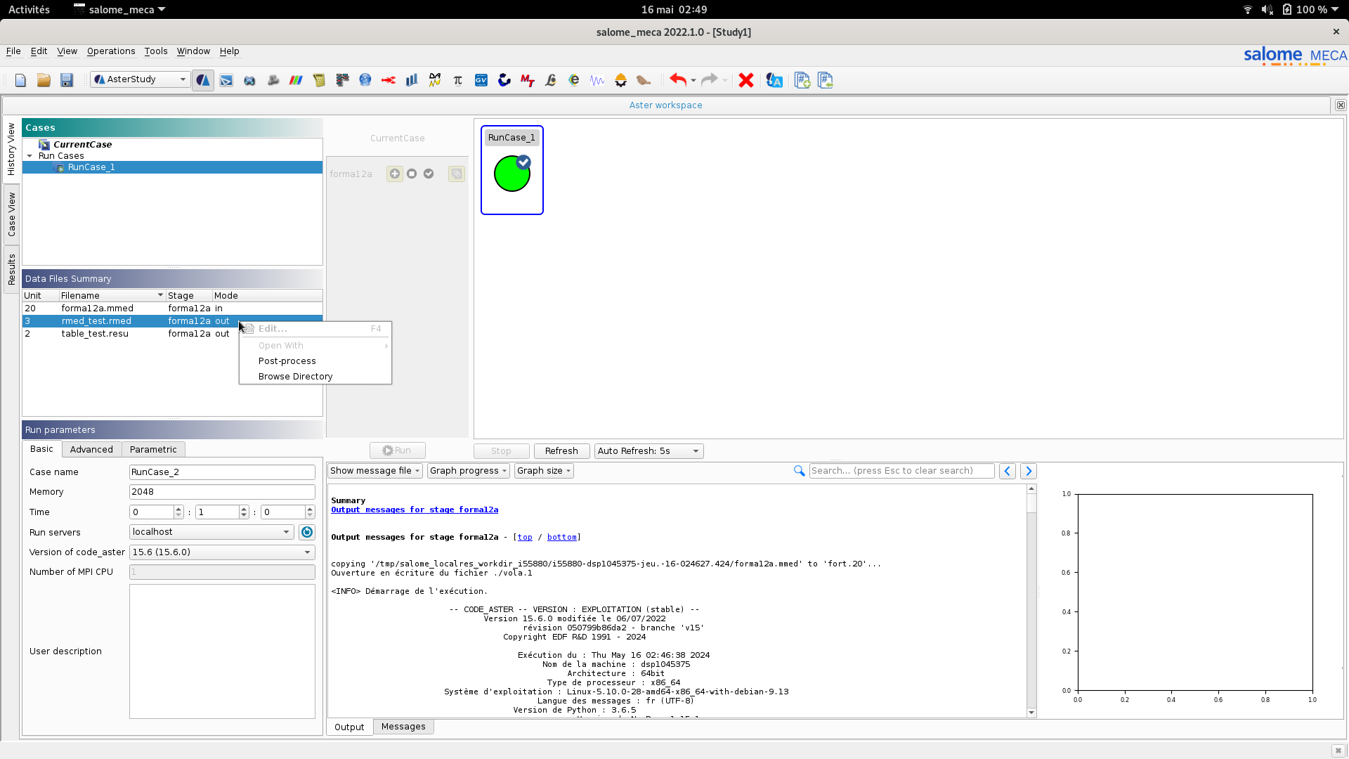
Fig. 2.9 Run via AsterStudy

Fig. 2.10 Calculation start parameter

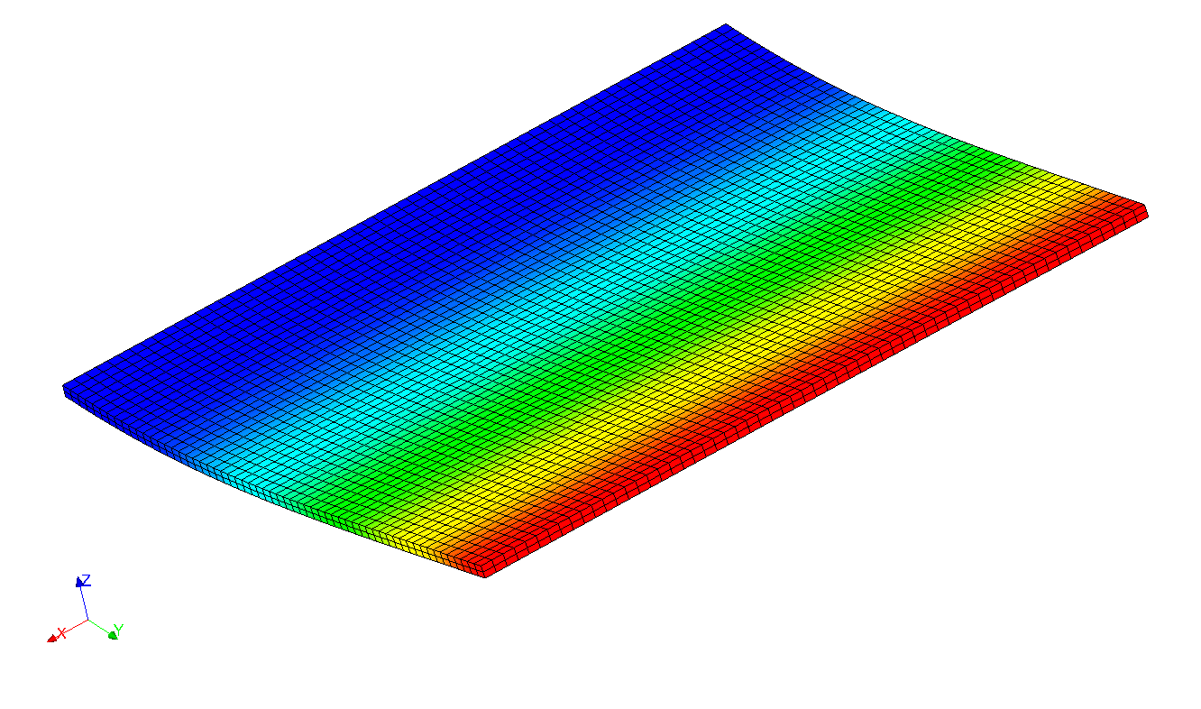
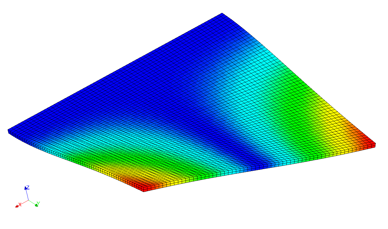
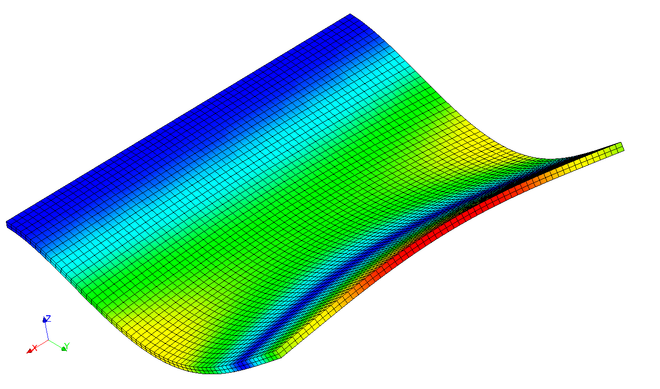
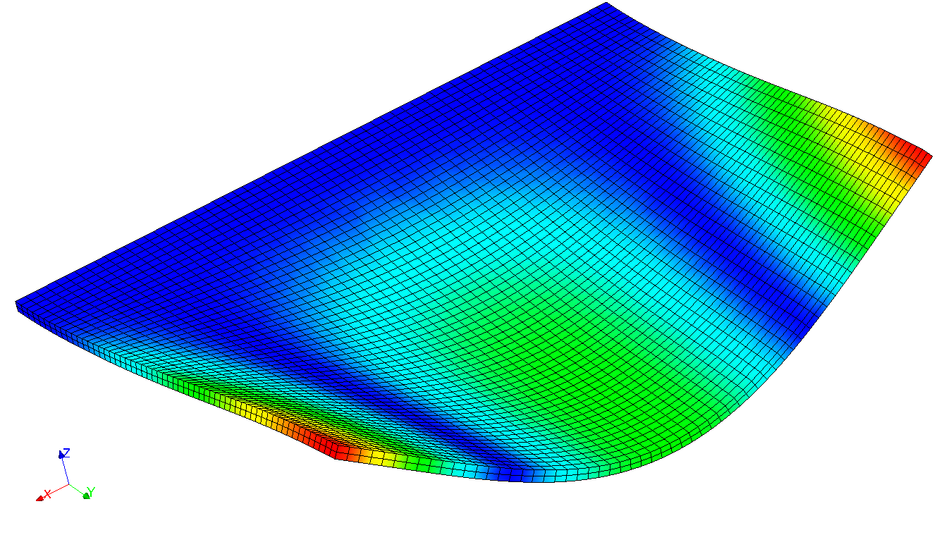
As an example, here are some modal deformations:

Figure 1: First mode (6.3 Hz)	Figure 2: Second mode (15.4 Hz)
Figure 3: Third mode (38.6 Hz)	Figure 4: Fourth Mode (49.0 Hz)

To check the quality of the mesh, it is, of course, possible to carry out a convergence study as a function of the fineness of the mesh. But on such simple geometry, it is possible to find a good approximation using an analytical formula (for example in*Formulas for Stress, Strain, and Structural Matrixes,* Walter D. Pikey — edited. John Wiley & Sons, Inc. 1994).

In the case studied, we find:

\(\mathit{f1}\mathrm{=}6.23\mathit{Hz}\)

\(\mathit{f3}\mathrm{=}38.16\mathit{Hz}\)

The results given by Code_Aster are therefore quite accurate, despite the coarseness of the mesh.

With a linear mesh, the results would not have been as good.