6. E-modeling — nonlinear dynamics#
The main objective of this TP is to set up a transient non-linear calculation taking into account plasticity. We are going to use the DYNA_NON_LINE operator.
6.1. Calculation procedure#
To calculate dynamic nonlinear behavior, we use the general-purpose operator DYNA_NON_LINE. It is close to STAT_NON_LINE and its use is close. The main difference is the time integration pattern and the influence of inertia and damping.
6.1.1. General data#
Compared to the previous calculations in DYNA_VIBRA and DYNA_LINE, the fundamental difference is that the matrices (stiffness, damping, and mass) and the second members (loads) are not to be calculated before the operator. In fact, the DYNA_NON_LINE command is said to be « monolithic » because the stiffness matrix varies during the transition since a non-linear problem (which depends on the displacement) is solved. You must therefore give him the information as you do in the macro command ASSEMBLAGE so that he can evaluate his operators himself:
CHAM_MATER
MODELE
possibly* CARA_ELEM * if you have structural elements or discretes (which is not the case here)
The loads are the same as in the previous years. They are given by the keyword factor EXCIT as in DYNA_VIBRA. Don’t forget to apply the sinus in FONC_MULT for gravity.
6.1.2. Choice of non-linear behavior#
The choice of non-linear behavior is made in the keyword factor COMPORTEMENT of DYNA_NON_LINE. If you do not enter anything, we will consider that the calculation is elastic in small deformations.
Of course, if you have non-linear behavior, you need to define the appropriate material characteristics in DEFI_MATERIAU.
In this exercise, we suggest von Mises plasticity with linear kinematic work hardening:
in* DEFI_MATERIAU , you have to choose ECRO_CINE . We propose D_SIGM_EPSI = 2GPa (Young’s modulus divided by 100) and an elastic limit SY = 20 0MPa. It is highly recommended to always enter the keyword ELAS *, even when doing plasticity.
in* DYNA_NON_LINE/COMPORTEMENT , we choose RELATION = “VMIS_CINE_LINE” and DEFORMATION =” PETIT “ . *
6.1.3. Choice of the time scheme and time discretization#
The choice of the time pattern is fundamental in dynamics. Moreover, a non-linear problem adds an additional constraint on time discretization in order to have sufficient precision for the integration of nonlinearity at the Gauss point level (plasticity). In code_aster, the majority of discretization schemes for behavioral equations are implicit and precise, but this precision may depend on this discretization, in particular because it makes some assumptions about the nature of the problem (see advanced code_aster training). It is therefore an additional numerical parameter that must be paid close attention to.
It is appropriate to choose a temporal discretization that has three characteristics:
compatible with the load applied. Care must be taken to have enough time discretization points to properly capture this load. The application of the Shannon rule is a good basis: at least a discretization frequency twice as high as that of the most penalizing load
temporal discretization must also be chosen according to the characteristics of the pattern in time: stability condition (for schemes that have one) and precision
Temporal discretization must be chosen to precisely integrate the non-linear part
It is proposed to take a time step of 0.002 s. Since the non-linear calculation is potentially very long, it is recommended to stop at time tfin = 0.1 s:
LISTR = DEFI_LIST_REEL (DEBUT =0. , INTERVALLE =_F (JUSQU_A =0.1, PAS =0.002,),)
The additional constraint of non-linear behavior imposes possibly allowing DYNA_NON_LINE to cut the time step when it fails to integrate. To do this, we use the DEFI_LIST_INST operator:
LIS = DEFI_LIST_INST (METHODE =” MANUEL “, DEFI_LIST =_F (LIST_INST = LISTR,),),
This command says that the calculation will be timed based on the list of moments LISTR (and, for example, we will save all the calculation data at these times),
But that in case of a problem (failure to integrate the nonlinear for example), we allow him to split the time step into 5, via ECHEC =_F (SUBD_NIVEAU =5, SUBD_PAS_MINI =1e-5, =1e-5, SUBD_METHODE =1e-5, =” MANUEL “,),. The cut is recursive: it cuts into 5, if it fails, it cuts back into 5, etc. It will stop permanently (failure) as soon as it reaches a minimum step given by the parameter SUBD_PAS_MINI =1E-5.
The result of this command should be entered directly in the key word INCREMENT/LIST_INST of DYNA_NON_LINE. Be careful to choose LIS and not LISTR, otherwise the time step cutting in case of failure will not be activated.
In the SCHEMA_TEMPS keyword, you can select your pattern in time. By default, it is a Newmark schema on the go. This pattern is unconditionally stable and conserves energy. Other schemes are available, such as the dissipative diagram HHT, which makes it possible to attenuate the digital disturbances generated by high frequencies. Here we adopt diagram HHT with the parameter ALPHA =-0.1.
6.1.4. Post-treatment#
The nonlinear calculation is long and produces a lot of data by default. Indeed, in non-linear mode, not only will you have access to displacements, speeds and accelerations (DEPL, VITE and ACCE) but also to the constraints at Gauss points (SIEF_ELGA) and to internal variables (VARI_ELGA) and to internal variables (* ). Over long transitions, the data produced can be very large. It is therefore recommended that you use the keyword ARCHIVAGE * to select when you want your data.
As we want to test the effect of plasticity, we will calculate the field SIEQ_ELGA in CALC_CHAMP to check the stress level (von Mises criterion). Moreover, we also test the hypothesis DEFORMATION =” PETIT “ by calculating the field EPEQ_ELGA in CALC_CHAMP.
Finally, for comparison purposes, it is possible to extract displacements, velocities and accelerations at the point P of the structure using the RECU_FONCTION command:
DEPL_DZ = RECU_FONCTION (GROUP_NO =”P”, NOM_CHAM =” DEPL “, NOM_CMP =”DZ”, RESULTAT = DYNADNL)
This function is then printable by IMPR_FONCTION.
It can also be done in the AsterStudy post-process module or in Paravis.
6.2. Analysis of the results — Newmark diagram#
Reading the « .mess » message file, we observe that the number of iterations increases when the material enters a non-linear domain, a contrario linear elastic steps, where convergence occurs in a single iteration.
On the transient, we have the following curves for the displacement, speed and acceleration at point P of the structure with the Newmark and HHT diagrams:
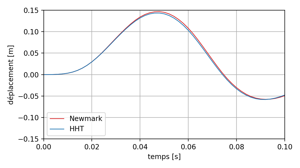
Fig. 6.1 Comparison of displacements between two schemes: Newmark and HHT#
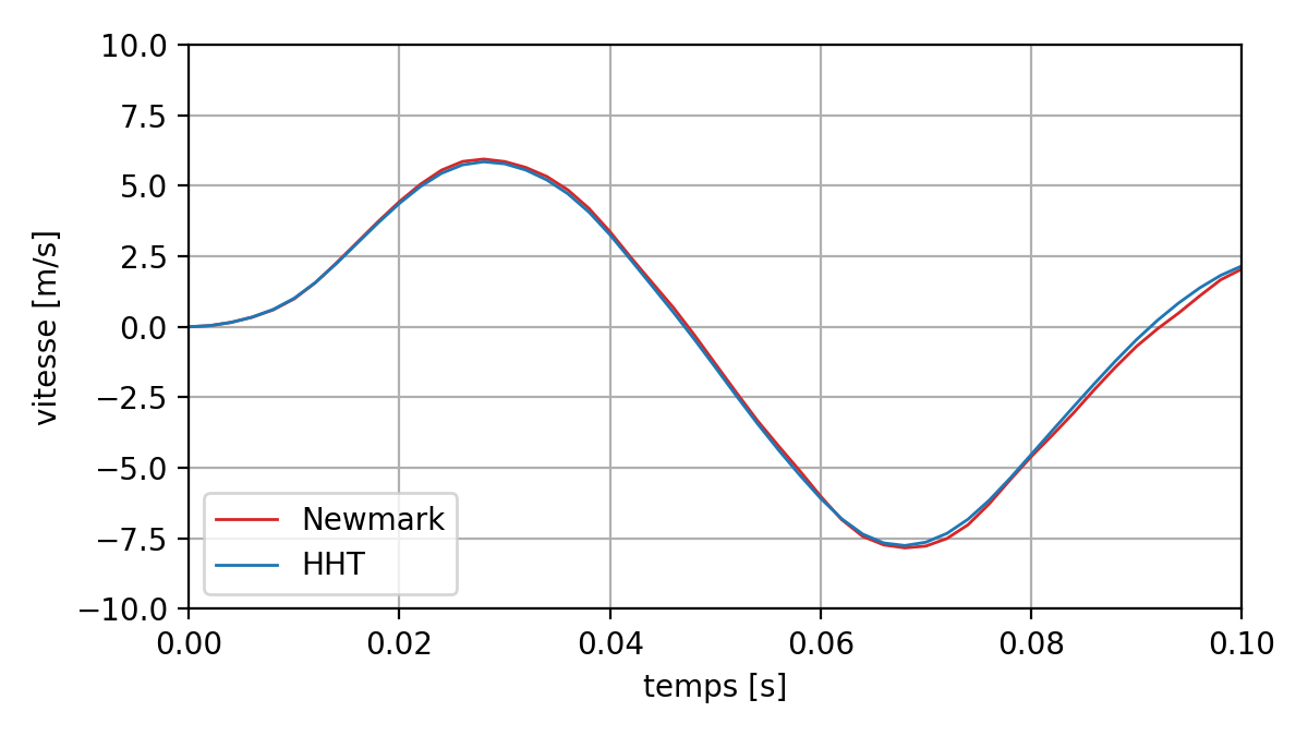
Fig. 6.2 Comparing speeds between two Newmark and HHT schemes#
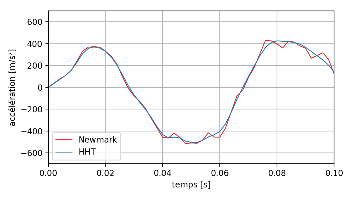
Fig. 6.3 Comparing accelerations between two Newmark and HHT schemes#
We can see that with the Newmark scheme the acceleration is disturbed by high-frequency effects. Figure HHT makes it possible to correct these problems a bit. The rest of the results correspond to the calculations carried out with diagram HHT.
The following curves show the effect of plasticity on the movement, speed, and acceleration of point P.
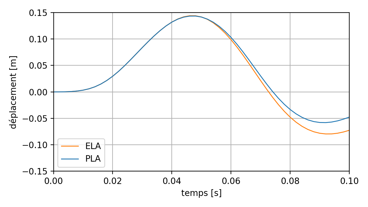
Fig. 6.4 Effect of plasticity on the displacement response of the point P#
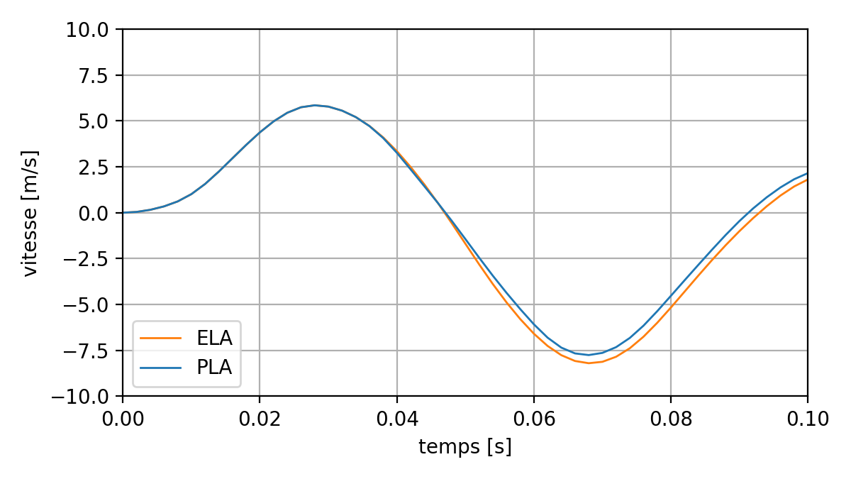
Fig. 6.5 Effect of plasticity on the speed response of the P point#
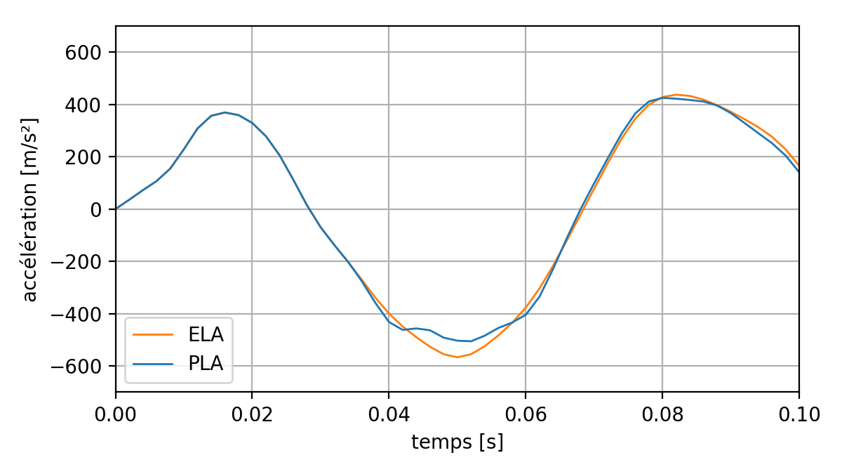
Fig. 6.6 Effect of plasticity on the acceleration response of the P point#
It is observed that, compared to elastic calculation: * plasticity « dampens » the amplitude of the response; * the apparent frequency of the structure decreases slightly.
These observations are a sign of the relaxation of the structure under the effect of plasticity, which can be verified by the evolution of the first natural frequency of the structure, obtained with the keyword MODE_VIBR =_F (LIST_INST = LISTR, NMAX_FREQ =1, =1, MATR_RIGI =” TANGENTE “, OPTION =” PLUS_PETITE”):
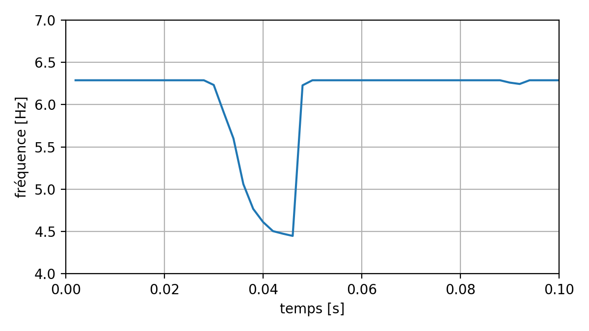
Fig. 6.7 Evolution of the frequency of the first mode in transient#
The following figure shows the maximum value of the equivalent von Mises stress over time, among all the gauss points in the set of elements of the structure. The constraint is capped at 200 MPa for plastic analysis.
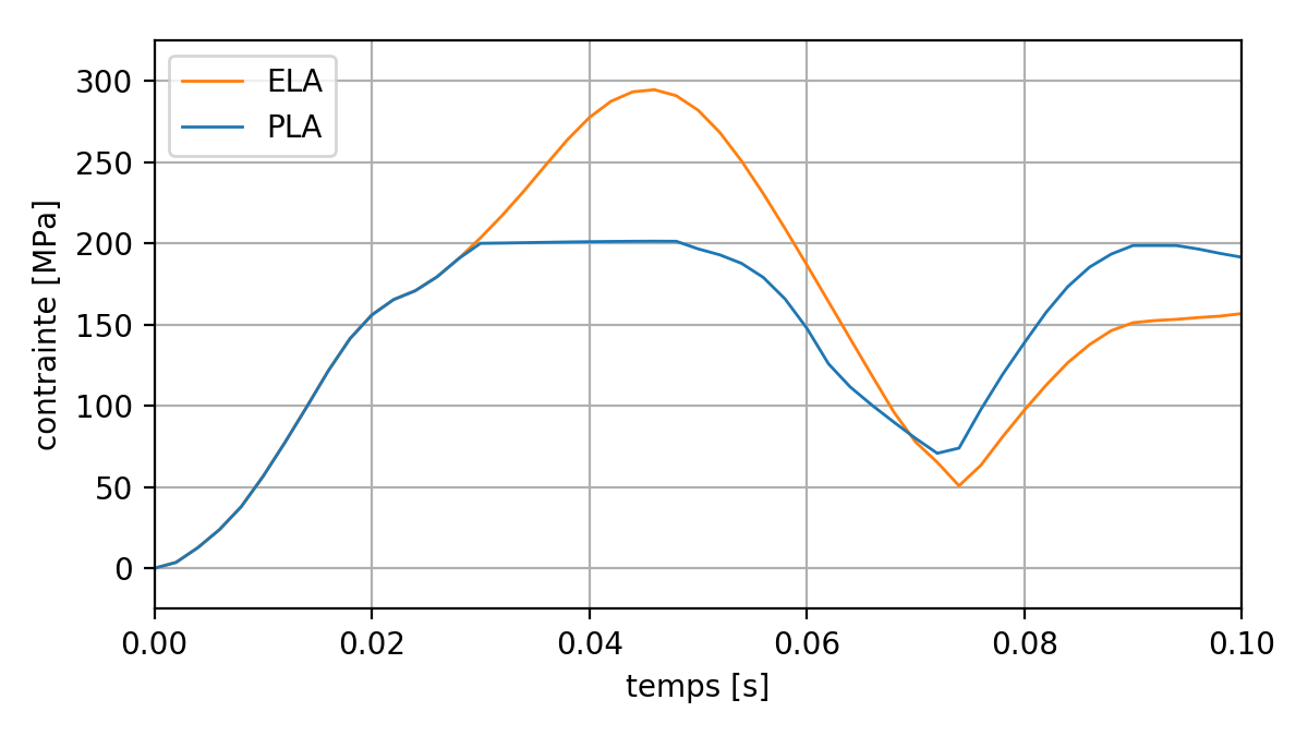
Fig. 6.8 Effect of plasticity on von Mises stress during the transition#
It is verified that the hypothesis of small deformations is correct. The following figure shows the maximum value of the second invariant of the strain tensor (EPEQ_ELGA/INVA_2) over time, among all the gauss points in the set of elements of the structure:
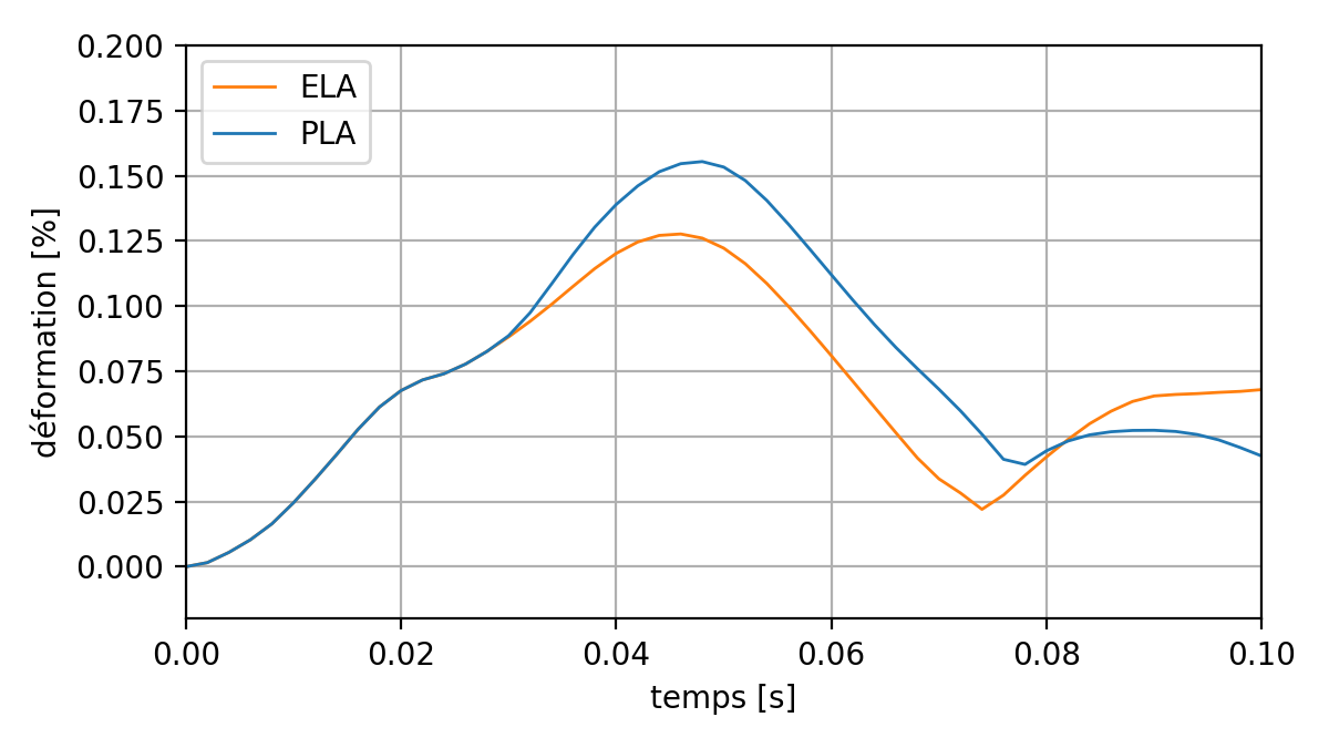
Fig. 6.9 Effect of plasticity on deformation during the transition#
The maximum deformation value is less than 0.2%. We are indeed in small deformations.
In general, in dynamics, it is recommended to look at the energy balance. To do this, we can activate the calculation of the quantities of energy during the entire transition using the keyword ENERGIE in DYNA_NON_LINE. It is possible to retrieve the energy balance after the calculation in a table. You have to use the command RECU_TABLE:
tableNRJ = RECU_TABLE (CO= DYNADNL, NOM_TABLE =” PARA_CALC “)
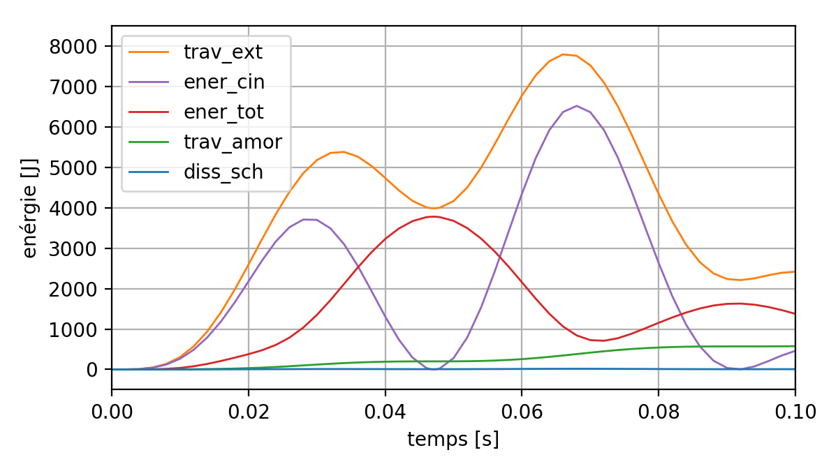
Fig. 6.10 Energy balance during the transition#
The maximum value of the dissipation of the temporal integration scheme HHT reached throughout the transient was less than 20 J. The scheme HHT adopted therefore made it possible to partially correct the high-frequency disturbances observed with the Newmark scheme, while maintaining negligible dissipation.