5. Special straight beams#
In this chapter, it is a question of taking into account straight beams whose cross section has properties that have been ignored until now, in particular beams with an offset center of torsion with respect to the neutral axis (the section does not have 2 axes of symmetry), and those whose cross section evolves continuously on their axis.
5.1. Eccentricity of the torsional axis in relation to the neutral axis#
The center of torsion is the point that remains fixed when the section is subjected to the torsional moment alone. It is also called the center of shear because a force applied at this point does not produce rotation \({\theta }_{x}\)
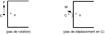
Figure 5.1-a: Section with center of torsion.
At point \(C\), the effects of bending and twisting are decoupled, so we can use the results established in the previous chapter. We find the components of displacement at point \(O\) by considering the rigid body relationship:
\(\overrightarrow{u}(O)=\overrightarrow{u}(C)+\overrightarrow{\mathrm{OC}}\wedge \overrightarrow{\Omega }\)
with \(\Omega =(\begin{array}{c}{\theta }_{x}\\ 0\\ 0\end{array})\) rotation vector and \(\overrightarrow{\mathrm{OC}}=(\begin{array}{c}0\\ {e}_{y}\\ {e}_{z}\end{array})\) the position of the center of torsion in the local coordinate system of the beam. In fact, we get:
\(\{\begin{array}{c}{u}_{x}={u}_{{x}_{c}}\\ {u}_{y}={u}_{{y}_{c}}+{e}_{z}{\theta }_{x}\\ {u}_{z}={u}_{{z}_{c}}-{e}_{y}{\theta }_{x}\end{array}\) [5.1-1]
The change in variables given by [eq] is written in matrix form:
\((\begin{array}{c}{u}_{{x}_{{c}_{1}}}\\ {u}_{{y}_{{c}_{1}}}\\ {u}_{{z}_{{c}_{1}}}\\ {\theta }_{{x}_{{c}_{1}}}\\ {\theta }_{{y}_{{c}_{1}}}\\ {\theta }_{{z}_{{c}_{1}}}\\ {u}_{{x}_{{c}_{2}}}\\ {u}_{{y}_{{c}_{2}}}\\ {u}_{{z}_{{c}_{2}}}\\ {\theta }_{{x}_{{c}_{2}}}\\ {\theta }_{{y}_{{c}_{2}}}\\ {\theta }_{{z}_{{c}_{2}}}\end{array})=(\begin{array}{cccccccccccc}1& 0& 0& 0& 0& 0& & & & & & \\ 0& 1& 0& -{e}_{z}& 0& 0& & & & & & \\ 0& 0& 1& {e}_{y}& 0& 0& & & & 0& & \\ 1& 0& 0& 1& 0& 0& & & & & & \\ 1& 0& 0& 0& 1& 0& & & & & & \\ 1& 0& 0& 0& 0& 1& & & & & & \\ & & & & & & 1& 0& 0& 0& 0& 0\\ & & & & & & 0& 1& 0& -{e}_{z}& 0& 0\\ & & 0& & & & 0& 0& 1& {e}_{y}& 0& 0\\ & & & & & & 0& 0& 0& 1& 0& 0\\ & & & & & & 0& 0& 0& 0& 1& 0\\ & & & & & & 0& 0& 0& 0& 0& 1\end{array})\begin{array}{c}(\begin{array}{c}{u}_{{x}_{{}_{1}}}\\ {u}_{{y}_{{}_{{}_{1}}}}\\ {u}_{{z}_{{}_{1}}}\\ {\theta }_{{x}_{{}_{1}}}\\ {\theta }_{{y}_{{}_{1}}}\\ {\theta }_{{z}_{{}_{1}}}\\ {u}_{{x}_{{}_{2}}}\\ {u}_{{y}_{{}_{2}}}\\ {u}_{{z}_{{}_{2}}}\\ {\theta }_{{x}_{{}_{2}}}\\ {\theta }_{{y}_{{}_{2}}}\\ {\theta }_{{z}_{{}_{2}}}\end{array})\end{array}\)
It is therefore sufficient to determine the elementary matrices of mass \(({M}_{c})\) and stiffness \(({K}_{c})\) in the coordinate system \((C,x,y,z)\) where the flexure and torsional movements are decoupled and then to transport themselves into the coordinate system linked to the neutral axis \((O,x,y,z)\) by the following transformations:
\(\begin{array}{}K={P}^{\text{T}}{K}_{c}P\\ \text{et}M={P}^{\text{T}}{M}_{c}P\end{array}\)
The values of \({e}_{y}\) and \({e}_{z}\) are to be provided to*Code_Aster* via the operand SECTION: “GENERALE” of the AFFE_CARA_ELEM operator, the values by default being obviously null values.
5.2. Variable sections#
It is possible to take into account continuously evolving sections for Timoshenko and Euler straight beams (POU_D_E and POU_D_T only). A distinction is made between two types of cross-section variation:
linear or refined,
quadratic or homothetic.
The distinction between the two types is easily understood using the example of a rectangular beam:
if only one of the lateral dimensions varies, we assume linearly, then the area of the straight section varies linearly, and is given by:
\(S(x)={S}_{1}\left[1+(\frac{{S}_{2}}{{S}_{1}}-1)\frac{x}{L}\right]\)
when the two lateral dimensions vary (linearly), the area of section will evolve quadratically.
\(S(x)={S}_{1}{\left[1+(\sqrt{\frac{{S}_{2}}{{S}_{1}}}-1)\frac{x}{L}\right]}^{2}\)
Code_Aster allows you to deal with “CERCLE”, “RECTANGLE” and “GENERALE” sections, but for obvious reasons of geometry, all these types of sections cannot accept both types of variation. The following table summarizes the possibilities that exist.
Section |
Constant |
Linear or Refine |
Quadratic or Homothetic |
circle |
yes |
no |
yes |
rectangle |
yes |
yes - according to y |
yes |
general |
yes |
no |
yes |
For the “RECTANGLE” section, the user chooses the type of variation, by specifying “AFFINE” or “HOMOTHÉTIQUE” in AFFE_CARA_ELEM. It should be noted that in the case “AFFINE”, the dimensions can only vary according to y.
In the case of circular hollow sections, for the section to be considered homothetic, it is necessary that \(\mathit{EP1}/\mathit{R1}=\mathit{EP2}/\mathit{R2}\). In the case of non-compliance with homothety the solution given by*Code_Aster* is approximated.
In general, we consider that the section varies according to the formula [eq]:
\(S(x)={S}_{1}{(1\text{+c}\frac{x}{L})}^{m}\) [5.2-1]
\({S}_{1}\) is the initial section in \(x=0\)
\(c\) is fixed by knowing the final section \({S}_{2}\) in \(x=L\).
\(m\) gives the degree of variation: \(m=1\) linear variation, \(m=2\) quadratic variation.
As the section varies, so do inertias \({I}_{y}(x)\), \({I}_{z}(x)\), and \({I}_{p}(x)\).
So we will have:
\({I}_{y}(x)={I}_{{y}_{1}}{(1\text{+c}\frac{x}{L})}^{\text{m+}2}\) [5.2-2]
\({I}_{z}(x)={I}_{{z}_{1}}{(1\text{+c}\frac{x}{L})}^{\text{m+}2}\) [5.2-3]
\({I}_{p}(x)={I}_{{p}_{1}}{(1\text{+c}\frac{x}{L})}^{\text{m+}2}\) [5.2-4]
\(c\) is determined for each formula based on the value for \({\text{x = L : I}}_{{y}_{2}}{\text{, I}}_{{z}_{2}}{\text{, I}}_{{p}_{2}}\).
The Young \((E)\) and Coulomb \((G)\) moduli are assumed to be constant.
The principle adopted by*Code_Aster* consists in calculating equivalent cross-section characteristics, which are constant on the beam, from the real characteristics given at both ends. These equivalent characteristics therefore depend on the phenomenon to which they contribute; in particular, they are distinct for the effects of rigidity or inertia.
5.2.1. Calculation of the stiffness matrix#
5.2.1.1. Determination of the equivalent cross section (\({S}_{\mathrm{eq}}\))#
The determination of the equivalent section does not use either the method taken in [§ 4.1.1] to obtain the exact stiffness matrix or an approximation of the solution by a polynomial function as described in [§ 4.1.4]. In fact, the method used differs from the finite element method and even from the Galerkin method; it consists in solving the problem of the variable-section beam without imposed distributed forces, which makes it possible to explain the forces at the ends as a function of the movements. This method is « consistent » with that of [§ 4.1.1] because the test functions defined in [§ 4.1.1] are equal to 1 or 0 on the ends of the beam, so [eq] nodal forces can be « assimilated » to efforts.
Moreover, this method makes it possible to obtain exact results for the static problem without distributed force and leads, as we will see, to a value \({S}_{\mathrm{eq}}\) between \({S}_{1}\) and \({S}_{2}\) which, in the general case, guarantees the convergence of the approximate solution to the exact solution (without however knowing the order of convergence).
Since the cross section of the beam is variable, the traction-compression equation in statics without imposed distributed effort is written:
\(\frac{\partial }{\partial x}\left[ES(x)\frac{\partial u}{\partial x}\right]=0\) [5.2.1.1-1]
with \(N(x)=ES(x)\frac{\partial u}{\partial x}\)
We determine the stiffness matrix in the general case [eq], we then deduce the values of the equivalent sections for cases \(m=1\) (linear progression) and \(m=2\) (quadratic progression).
By integrating [eq], we have:
\(\text{E S}(x)\frac{\partial u}{\partial x}={C}_{1}\)
or, taking into account the expression in \(S(x)\):
\(E{S}_{1}{(1\text{+c}\frac{x}{L})}^{m}\frac{\partial u}{\partial x}={C}_{1}\)
The integration constant is determined from the axial force values at the nodes.
We are integrating again in order to obtain the efforts at the nodes according to the movements \(u(0)={u}_{1}\) and \(u(L)={u}_{2}\):
\(\frac{\partial u}{\partial x}=\frac{{C}_{1}}{E{S}_{1}}{(1\text{+c}\frac{x}{L})}^{-m}\)
Where \(\text{u}(x)=\frac{{C}_{1}}{E{S}_{1}}\frac{L}{c}\text{ln}(1\text{+c}\frac{x}{L}){\text{+C}}_{2}\text{}\) if \(m=1\)
and \(u(x)=\frac{{C}_{1}}{E{S}_{1}}\frac{L}{c}\frac{1}{(l-m){(1+c\frac{x}{L})}^{m-1}}+{C}_{2}\) if \(m\ge 2\)
We can see that the expression for \(u(x)\) is far from being polynomial.
Taking into account the fact that:
\({C}_{1}=-{N}_{1}\) for \(x=0\)
\({C}_{1}=+{N}_{2}\) for \(x=L\)
and that:
\({C}_{2}=\frac{{(1\text{+c})}^{-m+1}\text{u}(0)-u(L)}{{(1\text{+c})}^{-m+1}-1}\)
We get:
for \(m=1\), \(\{\begin{array}{c}{N}_{1}=\frac{E{S}_{1}\text{c}}{\text{L}\text{ln}(1+c)}({u}_{1}-{u}_{2})\\ {N}_{2}=\frac{E{S}_{1}\text{c}}{\text{L}\text{ln}(1+c)}({u}_{2}-{u}_{1})\end{array}\)
and for \(m=2\), \(\{\begin{array}{c}{N}_{1}=\frac{E{S}_{1}\text{c}\left(1-m\right)}{L}\text{}\left[-{u}_{1}\left(\frac{{\left(1+c\right)}^{m-1}}{1-{\left(1+c\right)}^{m-1}}\right)+{u}_{2}\left(\frac{{\left(1+c\right)}^{m-1}}{1-{\left(1+c\right)}^{m-1}}\right)\right]\text{}\\ {N}_{2}=\frac{E{S}_{1}\text{c}\left(1-m\right)}{L}\text{}\left[{u}_{1}\left(\frac{{\left(1+c\right)}^{m-1}}{1-{\left(1+c\right)}^{m-1}}\right)-{u}_{2}\left(\frac{{\left(1+c\right)}^{m-1}}{1-{\left(1+c\right)}^{m-1}}\right)\right]\end{array}\)
By replacing \(c\) with its value, that is:
if \(m=1\),
\(\begin{array}{c}c=\frac{{S}_{2}}{{S}_{1}}-1\text{,}\\ \text{}{N}_{1}=\frac{E}{L}\frac{\left({S}_{2}-{S}_{1}\right)}{\text{ln}{\text{S}}_{2}-\text{ln}{\text{S}}_{1}}\left({u}_{1}-{u}_{2}\right)\\ \text{}{N}_{2}=\frac{E}{L}\frac{\left({S}_{2}-{S}_{1}\right)}{\text{ln}{\text{S}}_{2}-\text{ln}{\text{S}}_{1}}\left({u}_{2}-{u}_{1}\right)\end{array}\)
if \(m=2\),
\(\begin{array}{c}\text{}\text{c}=\sqrt{\frac{{S}_{2}}{{S}_{1}}}-1\\ {\text{N}}_{1}=\frac{E}{L}\sqrt{{S}_{1}{\text{S}}_{2}}\left({u}_{1}-{u}_{2}\right)\\ {\text{N}}_{2}=\frac{E}{L}\sqrt{{S}_{1}{\text{S}}_{2}}\left({u}_{2}-{u}_{1}\right)\end{array}\)
We note that the stiffness matrices, in the two cases treated, will have the same shape as for a constant cross section if we take as equivalent cross section:
\({S}_{\text{eq}}=\frac{({S}_{2}-{S}_{1})}{\text{ln}{S}_{2}-\text{ln}{\text{S}}_{1}}\) for a linearly varying cross section
\({S}_{\text{eq}}=\sqrt{{S}_{1}{S}_{2}}\) for a quadratically varying section
5.2.1.2. Determination of an equivalent torsional constant (Ceq)#
The pure torsional equation for a beam with variable cross section is written as:
\(\frac{\partial }{\partial x}(\text{G C}(x)\frac{\partial {q}_{x}}{\partial x})=0\) [5.2.1.2-1]
with \(C(x)={C}_{1}{(1+\text{c}\frac{x}{L})}^{m+2}\) (\(m=1\) or \(2\))
The method is the same as for calculating the equivalent section: the aim is to integrate the previous equation in order to obtain the forces (torsional torques \({\Gamma }_{{x}_{1}}\text{,}{\Gamma }_{{x}_{2}}\)) as a function of the displacements at the nodes \(({\theta }_{{x}_{1}},{\theta }_{{x}_{2}})\) and to deduce, by comparison with the formulas with a constant section, the expression of an equivalent polar geometric moment.
By integrating [eq], we have:
\({\text{G C}}_{1}{(1+c\frac{x}{L})}^{m+2}\frac{\partial {\theta }_{x}}{\partial x}={D}_{1}\),
\({D}_{1}\) the integration constant is determined by the torsional torques applied to the nodes.
From: |
\(\frac{\partial {\theta }_{x}}{\partial x}=\frac{{D}_{1}}{{\text{G C}}_{1}}{(1+c\frac{x}{L})}^{-(m+2)},\) |
We deduce: |
\({\theta }_{x}(x)=\frac{{D}_{1}}{{\text{G C}}_{1}}\frac{-L}{\text{c}(\text{m+}1)}{(1+c\frac{x}{L})}^{-(m+1)}+{D}_{2}\) |
We determine \({D}_{2}\) from the system:
\(\{\begin{array}{c}{\theta }_{{x}_{1}}=\frac{-{D}_{1}L}{{\mathrm{GC}}_{1}c(m+1)}+{D}_{2}\\ {\theta }_{{x}_{2}}=\frac{-{D}_{1}L}{{\mathrm{GC}}_{1}c(m+1)}{(1+c)}^{-(m+1)}+{D}_{2}\end{array}\)
That is: \({D}_{2}=\frac{{\theta }_{{x}_{1}}{(1+c)}^{-(m+1)}+c{\theta }_{{x}_{2}}}{{(1+c)}^{-(m+1)}-1}\)
Taking into account the fact that:
\({D}_{1}=-{\Gamma }_{1}\) for \(x=0\)
\({D}_{1}={\Gamma }_{2}\) for \(x=L\)
we finally have:
for \(m=1\),
\(\begin{array}{}\{\begin{array}{c}{\Gamma }_{1}=\frac{G}{L}\frac{2({C}_{2}{C}_{1}^{\frac{2}{3}}-{C}_{1}{C}_{2}^{\frac{2}{3}})}{({C}_{2}^{\frac{2}{3}}-{C}_{1}^{\frac{2}{3}})}({\theta }_{{x}_{1}}-{\theta }_{{x}_{2}})\\ {\Gamma }_{2}=\frac{G}{L}\frac{2({C}_{2}{C}_{1}^{\frac{2}{3}}-{C}_{1}{C}_{2}^{\frac{2}{3}})}{({C}_{2}^{\frac{2}{3}}-{C}_{1}^{\frac{2}{3}})}({\theta }_{{x}_{2}}-{\theta }_{{x}_{1}})\end{array}\end{array}\)
Therefore, in the case of a linearly varying section, we take an equivalent geometric polar moment \({C}_{\mathrm{eq}}\) of the following form:
\({C}_{\text{eq}}=\frac{2({C}_{2}{C}_{1}^{\frac{2}{3}}-{C}_{1}{C}_{2}^{\frac{2}{3}})}{({C}_{2}^{\frac{2}{3}}-{C}_{1}^{\frac{2}{3}})}\) linear variation
for \(m=2\),
\(\{\begin{array}{}{\Gamma }_{1}=\frac{G}{L}\frac{3({C}_{2}{C}_{1}^{\frac{3}{4}}-{C}_{1}{C}_{2}^{\frac{3}{4}})}{({C}_{2}^{\frac{3}{4}}-{C}_{1}^{\frac{3}{4}})}({\theta }_{{x}_{1}}-{\theta }_{{x}_{2}})\\ {\Gamma }_{2}=\frac{G}{L}\frac{3({C}_{2}{C}_{1}^{\frac{3}{4}}-{C}_{1}{C}_{2}^{\frac{3}{4}})}{({C}_{2}^{\frac{3}{4}}-{C}_{1}^{\frac{3}{4}})}({\theta }_{{x}_{2}}-{\theta }_{{x}_{1}})\end{array}\)
In the case of a cross section varying quadratically, the polar geometric moment is written as:
\({C}_{\text{eq}}=\frac{3({C}_{2}{C}_{1}^{\frac{3}{4}}-{C}_{1}{C}_{2}^{\frac{3}{4}})}{({C}_{2}^{\frac{3}{4}}-{C}_{1}^{\frac{3}{4}})}\) quadratic variation
5.2.1.3. Determination of equivalent geometric moments#
In fact, it does not seem possible to find, as we did for the section or the polar geometric moment, equivalent geometric moments \(({I}_{{y}_{\text{eq}}}\text{et}{I}_{{z}_{\text{eq}}})\) that would replace the geometric moments \(({I}_{y}\text{et}{I}_{z})\) in the expression of the terms of the stiffness matrix.
Here we present the method proposed by J.R. BANERJEE and F.W. WILLIAMS [bib 3] which explain the stiffness matrix in the case of a flexural movement of an Euler-Bernoulli beam with variable cross section (linear or quadratic).
The results correspond to those programmed in Code_Aster for an Euler-Bernoulli beam with variable cross section (linear or quadratic). By extension, the same approach is applied to Timoshenko beams. The results are not detailed here.
Let us consider the bending in plane \((xoy)\).
Starting from the static equation of the flexural motion of an Euler-Bernoulli type beam:
\(\frac{{\partial }^{2}}{\partial {x}^{2}}\left[{\text{EI}}_{z}(x)\frac{{\partial }^{2}v}{\partial {x}^{2}}\right]=0\text{}\), and \({\theta }_{z}=\frac{\partial v}{\partial x}\)
\(v(x)\) is expressed in terms of four integration constants \(({C}_{1}\text{,}{C}_{2}\text{,}{C}_{3}\text{,}{C}_{4})\). These constants are determined by the values of the displacements at the nodes:
\(\begin{array}{}v(o)={v}_{1}\text{}\text{}\text{v}(L)={v}_{2}\\ {\theta }_{z}(o)={\theta }_{{z}_{1}}{\theta }_{z}(L)={\theta }_{{z}_{2}}\end{array}\)
that is: \((\begin{array}{c}{v}_{1}\\ {\theta }_{{z}_{1}}\\ {v}_{2}\\ {\theta }_{{z}_{2}}\end{array})=\text{B}(\begin{array}{c}{C}_{1}\\ {C}_{2}\\ {C}_{3}\\ {C}_{4}\end{array})\), \(B\) matrix \((4\times 4)\).
The efforts: \({V}_{y}(x)=\frac{\partial }{\partial x}\left[{\text{EI}}_{z}(x)\frac{{\partial }^{2}v}{\partial {x}^{2}}\right]\)
and the moments: \({M}_{z}(x)={\text{EI}}_{z}(x)\text{}\frac{{\partial }^{2}v}{\partial {x}^{2}}\),
are also expressed in terms of these integration constants, and we can write:
\((\begin{array}{c}{T}_{{y}_{1}}\\ {M}_{{z}_{1}}\\ {T}_{{y}_{2}}\\ {M}_{{z}_{2}}\end{array})=D(\begin{array}{c}{C}_{1}\\ {C}_{2}\\ {C}_{3}\\ {C}_{4}\end{array})\), \(D\) matrix \((4\times 4)\).
The stiffness matrix corresponds to product \({\mathrm{DB}}^{-1}\). The terms of this matrix are explained in the following tables.
Recall that \({I}_{z}(x)={I}_{{z}_{1}}{(1+\text{c}\frac{x}{L})}^{m+2}\), \(m=1\) or \(2\),
Let’s say \({\text{W}}_{1}={\text{EI}}_{{z}_{1}}\frac{c}{L}{\text{, W}}_{2}={\text{EI}}_{{z}_{1}}{(\frac{c}{L})}^{2}{\text{, W}}_{3}={\text{EI}}_{{z}_{1}}{(\frac{c}{L})}^{3}\text{.}\)
Afinine variation |
Quadratic variation |
|
\(m=1\) |
|
|
\(c={(\frac{{I}_{2}}{{I}_{1}})}^{\frac{1}{3}}-1\) |
|
|
\({\Phi }_{1}\) |
|
|
\({\Phi }_{2}\) |
|
|
\({\Phi }_{3}\) |
|
|
\({\Phi }_{4}\) |
|
|
\({\Phi }_{5}=c{\Phi }_{2}-{\Phi }_{4}\) |
\(2\mathrm{c²}(c+1)\) |
|
\({\Phi }_{6}=c{\Phi }_{3}-{\Phi }_{5}\) |
\(4\mathrm{c²}(c+1)\) |
|
\(\Delta\) |
|
|
The matrix \(K\) is then written as:
\(\mathrm{K}=\frac{1}{\Delta }\text{}\left(\begin{array}{cccc}{W}_{3}{\Phi }_{1}& {W}_{2}{\Phi }_{2}& -{W}_{3}{\Phi }_{1}& {W}_{2}{\Phi }_{3}\\ & {W}_{1}{\Phi }_{4}& -{W}_{2}{\Phi }_{2}& +{W}_{1}{\Phi }_{5}\\ \text{Sym}& & {W}_{3}{\Phi }_{1}& -{W}_{2}{\Phi }_{3}\\ & & & {W}_{1}{\Phi }_{6}\end{array}\right)\)
Now let’s consider bending in plane \((xOz)\).
For sections with quadratic variation, the approach is identical. But it differs for linearly varying sections (following \(y\) only).
The terms of the stiffness matrix corresponding to the bending in plane \((\mathrm{0, }x,z)\) are calculated using the values given in the following table.
Affine variation: flexure in plane \((\mathrm{0,}x,z)\) |
|
\(c=(\frac{{I}_{2}}{{I}_{1}})-1\) |
|
\({\Phi }_{1}\) |
\(2\frac{\mathrm{ln}(c+1)}{c}\) |
\({\Phi }_{2}\) |
\(2-{\Phi }_{1}\) |
\({\Phi }_{3}\) |
\((c+1){\Phi }_{1}-2\) |
: label: EQ-None
{Phi} _ {5} =c {Phi} _ {2} - {Phi} _ {4}
|:math: `{\ Phi} _ {6} =c {\ Phi} _ {3} - {\ Phi} _ {5}` | | +--------------+--------------------------------+ |:math:`\Delta`|:math:`(c+2)mathrm{ln}(c+1)-2c`| +————–+——————————–+
In the case of Timoshenko beams, for the shear coefficients, the relationships used for the section are applied to the reduced section \(k\cdot S\), namely:
\(\begin{array}{c}{({k}_{y}S)}_{\mathrm{eq}}=\frac{({k}_{{y}_{2}}{S}_{2}-{k}_{{y}_{1}}{S}_{1})}{\mathrm{ln}({k}_{{y}_{2}}{S}_{2})-\mathrm{ln}({k}_{{y}_{1}}{S}_{1})}\\ {({k}_{z}S)}_{\mathrm{eq}}=\frac{({k}_{{z}_{2}}{S}_{2}-{k}_{{z}_{1}}{S}_{1})}{\mathrm{ln}({k}_{{z}_{2}}{S}_{2})-\mathrm{ln}({k}_{{z}_{1}}{S}_{1})}\end{array}\}\) if the variation is fine,
\(\begin{array}{}\begin{array}{c}{({k}_{y}\text{S})}_{\text{eq}}=\sqrt{{S}_{1}{\text{S}}_{2}{\text{k}}_{{y}_{1}}{\text{k}}_{{y}_{2}}}\\ {({k}_{z}\text{S})}_{\text{eq}}=\sqrt{{S}_{1}{\text{S}}_{2}{\text{k}}_{{z}_{1}}{\text{k}}_{{z}_{2}}}\end{array}\}\end{array}\) if the variation is quadratic,
and the additional terms are introduced in \(K\) in the same way as for a constant section. The calculations are not detailed here. We obtain a matrix \(K\) in the same shape as before with the main modification being the value of \(\Delta\):
affine variation:
\(\Delta =(c+2)\text{ln}(c+1)-\mathrm{2c}+\frac{{\Phi }^{2}}{\text{12}}{c}^{3}(c+2)\)
quadratic variation:
\(\Delta =\frac{{c}^{3}}{c+1}+\frac{{\Phi }^{2}}{3}{c}^{3}({c}^{2}+\mathrm{3c}+3)\)
5.2.2. Calculating the mass matrix#
5.2.2.1. By the method of equivalent masses#
« Average » values are calculated for the section, the reduced section, and the moments, namely:
\(S=\frac{{S}_{1}{\text{+S}}_{2}}{2}\text{}\) |
if the variation is fine |
\(S=\frac{1}{L}{\int }_{0}^{L}S(x)\text{dx}=\frac{{S}_{1}{\text{+S}}_{2}+\sqrt{{S}_{1}{\text{S}}_{2}}}{3}\) |
if the variation is quadratic |
\(\begin{array}{c}{I}_{y}=\frac{{I}_{{y}_{1}}+{I}_{{y}_{2}}}{2}\\ {I}_{z}=\frac{{I}_{{z}_{1}}+{I}_{{z}_{2}}}{2}\\ {I}_{{\theta }_{x}}=\rho \frac{{I}_{{y}_{1}}+{I}_{{y}_{2}}+{I}_{{z}_{1}}+{I}_{{z}_{2}}}{2}\end{array}\}\) |
regardless of the variation |
The mass matrix is then calculated as that of a beam having these characteristics.
5.2.2.2. By the concentrated mass method (diagonal matrix)#
If the cross section varies in a fine manner, the programmed matrices correspond, in terms of traction-compression and torsional movements, to those of beams with a constant section, using equivalent torsional sections and inertias:
◦ for tensile compression:
\(\rho L\left(\begin{array}{cc}\frac{{\mathrm{3S}}_{1}+{S}_{2}}{8}& 0\\ 0& \frac{{\mathrm{3S}}_{2}+{S}_{1}}{8}\end{array}\right)\)
◦ for twisting:
\(\rho \frac{L\left({I}_{{y}_{1}}+{I}_{{z}_{1}}+{I}_{{y}_{2}}+{I}_{{z}_{2}}\right)}{4}\left(\begin{array}{cc}1& 0\\ 0& 1\end{array}\right)\left(\begin{array}{c}{\theta }_{{x}_{1}}\\ {\theta }_{{x}_{2}}\end{array}\right)\)
◦ for flexure movements:
\(\left(\begin{array}{cccc}\frac{\rho {S}_{1}L}{2}& & & \\ & {M}_{\mathrm{5,5}}\left({M}_{\mathrm{6,6}}\right)& & 0\\ & & \frac{\rho {S}_{2}L}{2}& \\ & 0& & \\ & & & {M}_{\mathrm{11,11}}\left({M}_{\mathrm{12,12}}\right)\end{array}\right)\left(\begin{array}{c}\begin{array}{c}{v}_{1}\left({w}_{1}\right)\\ \end{array}\\ \begin{array}{c}{\theta }_{{z}_{1}}\left({\theta }_{{y}_{1}}\right)\\ \end{array}\\ \begin{array}{c}{v}_{2}\left({w}_{2}\right)\\ \end{array}\\ \begin{array}{c}{\theta }_{{z}_{2}}\left({\theta }_{{y}_{2}}\right)\\ \end{array}\end{array}\right)\)
with \({M}_{\mathrm{5,5}}={M}_{11.11}=\mathrm{min}\left(\frac{\rho {S}_{\mathit{eq}}{L}^{3}}{105},\frac{\rho {S}_{\mathit{eq}}{L}^{2}}{48}\right)+\frac{\rho L}{15}\left({I}_{{y}_{1}}+{I}_{{y}_{1}}\right)\)
\({M}_{\mathrm{6,6}}={M}_{\mathrm{12,12}}=\mathrm{min}\left(\frac{\rho {S}_{\mathit{eq}}{L}^{3}}{105},\frac{\rho {S}_{\mathit{eq}}{L}^{2}}{48}\right)+\frac{\rho L}{15}\left({I}_{{z}_{1}}+{I}_{{z}_{1}}\right)\) with \({S}_{\mathit{eq}}=\left(\frac{{S}_{1}+{S}_{2}}{2}\right)\)
If the section varies homothetically, the matrices are programmed, for the various movements, as follows:
◦ for traction-compression:
\((\begin{array}{cc}\rho \frac{(5{S}_{1}+{S}_{2})}{12}L& 0\\ 0& \rho \frac{({S}_{1}+5{S}_{2})}{12}L\end{array})(\begin{array}{c}\begin{array}{}{u}_{1}\\ \end{array}\\ \begin{array}{}{u}_{2}\\ \end{array}\end{array})\)
◦ for twisting:
\(\rho L\frac{({I}_{{y}_{1}}+{I}_{{y}_{2}}+{I}_{{z}_{1}}+{I}_{{z}_{2}})}{4}(\begin{array}{cc}1& 0\\ 0& 1\end{array})(\begin{array}{c}{\theta }_{{x}_{1}}\\ {\theta }_{{x}_{2}}\end{array})\)
◦ for bending in each of the two planes:
\(\left(\begin{array}{cccc}\rho \frac{\left(5{S}_{1}+{S}_{2}\right)}{12}L& & & \\ & {M}_{\mathrm{5,5}}\left({M}_{\mathrm{6,6}}\right)& & 0\\ & & \rho \frac{\left({S}_{1}+5{S}_{2}\right)}{12}L& \\ & & & {M}_{\mathrm{11,11}}\left({M}_{\mathrm{12,12}}\right)\end{array}\right)\left(\begin{array}{c}\begin{array}{c}{v}_{1}\left({w}_{1}\right)\\ \end{array}\\ \begin{array}{c}{\theta }_{{z}_{1}}\left({\theta }_{{y}_{1}}\right)\\ \end{array}\\ \begin{array}{c}{v}_{2}\left({w}_{2}\right)\\ \end{array}\\ \begin{array}{c}{\theta }_{{z}_{2}}\left({\theta }_{{y}_{2}}\right)\\ \end{array}\end{array}\right)\)
with \({M}_{\mathrm{5,5}}={M}_{\text{11},\text{11}}=\text{min}\left[\frac{\rho \left({S}_{1}+{S}_{2}\right)}{2}\frac{{L}^{3}}{\text{105}}\text{,}\frac{\rho \left({S}_{1}+{S}_{2}\right)}{2}\frac{{L}^{3}}{\text{48}}\right]+\rho \left({I}_{{y}_{1}}+{I}_{{y}_{2}}\right)\frac{L}{\text{15}}\)
and \({M}_{\mathrm{6,6}}={M}_{\text{12},\text{12}}=\text{min}\left[\frac{\rho \left({S}_{1}+{S}_{2}\right)}{2}\frac{{L}^{3}}{\text{105}}\text{,}\frac{\rho \left({S}_{1}+{S}_{2}\right)}{2}\frac{{L}^{3}}{\text{48}}\right]+\rho \left({I}_{{z}_{1}}+{I}_{{z}_{2}}\right)\frac{L}{\text{15}}\)