8. Curved beam#
Note: The curved beam element no longer exists in Code_Aster. To model a curved beam, you must mesh the curved part with enough straight elements: 20 to 40 straight elements for a 90° bend give completely satisfactory results.
This chapter is retained, because in the base of the test cases of Code_Aster structures that have bends are validated and compared to the theoretical solutions obtained with curved beam elements from the theory presented below.
To calculate the stiffness matrix for a curved beam element, we do the calculation by going through various steps.
We start from the integrated equilibrium equations that will give us a matrix (noted \({J}_{\theta }\)) to determine the forces at one point on the beam knowing the forces at another point. This matrix will take into account local base change.
Then, by writing the potential energy of the element and noting the decoupling of the flexure in the plane of the element from the flexure outside this plane, the two flexibility matrices are determined.
Finally, the flexibility matrices being calculated, the local stiffness matrix is obtained using the Castigliano principle, which must be recalculated in the global base in order to be assembled.
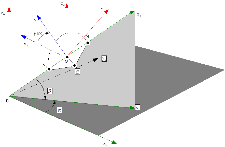
Figure 8-a : Local coordinate system for the curved beam.
To relate the forces applied at one point \(P\) of the structure to the forces obtained at another point \(Q\) of the structure, the static equilibrium equations of a curved beam are integrated (without distributed effort).
Here we will limit ourselves to studying the curved beam with a constant section (taking into account transverse shear) and with a constant radius of curvature.
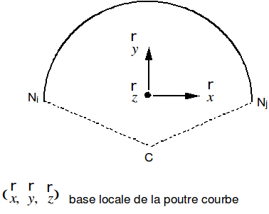
Figure 8-b : Average coordinate system (local coordinate system)
The static equilibrium equations are:
\(\begin{array}{cc}\{\begin{array}{c}{N}_{,s}-{V}_{1}=0\\ {V}_{\mathrm{1,}s}+\frac{N}{R}=0\\ {V}_{\mathrm{2,}s}=0\end{array}\text{}& \{\begin{array}{c}{M}_{T,s}-\frac{{M}_{1}}{R}=0\\ {M}_{\mathrm{1,}s}+\frac{{M}_{T}}{R}-{V}_{2}=0\\ {M}_{\mathrm{2,}s}+{V}_{1}=0\end{array}\end{array}\)
this for:
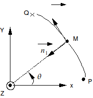
Figure 8-c : Curvilinear coordinate system.
To integrate, we use the conditions in \(P\):
\(\begin{array}{cc}\{\begin{array}{c}N={F}_{y}\\ {V}_{1}=-{\text{F}}_{x}\\ {V}_{2}={F}_{z}\end{array}\text{}& \{\begin{array}{c}{M}_{T}={M}_{y}\\ {M}_{1}=-{\text{M}}_{x}\\ {M}_{2}={M}_{z}\end{array}\end{array}\)
By integrating and passing into the following axis system:
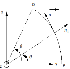
Figure 8-d : Axis system chosen by integration.
We get:
\(\left[\begin{array}{c}N\\ {V}_{1}\\ {V}_{2}\\ {M}_{T}\\ {M}_{1}\\ {M}_{2}\end{array}\right]=\underset{{J}_{\theta }}{\underset{\underbrace{}}{(\begin{array}{cccccc}\mathrm{cos}\theta & -\mathrm{sin}\theta & 0& 0& 0& 0\\ \mathrm{sin}\theta & \mathrm{cos}\theta & 0& 0& 0& 0\\ 0& 0& 1& 0& 0& 0\\ 0& 0& R(\mathrm{cos}\theta -1)& \mathrm{cos}\theta & -\mathrm{sin}\theta & 0\\ 0& 0& R\mathrm{sin}\theta & \mathrm{sin}\theta & \mathrm{cos}\theta & 0\\ R(\mathrm{cos}\theta -1)& -R\mathrm{sin}\theta & 0& 0& 0& 1\end{array})}}\left[\begin{array}{c}{F}_{x}\\ {F}_{y}\\ {F}_{z}\\ {M}_{x}\\ {M}_{y}\\ {M}_{z}\end{array}\right]\)
Now we are going to take into account the mechanical characteristics using potential energy:
\({E}_{p}=\frac{1}{2}\underset{{s}_{1}}{\overset{{s}_{2}}{\int }}(\frac{{\tilde{N}}^{2}}{ES}+\frac{{\tilde{V}}_{1}^{2}}{{k}_{1}SG}+\frac{{\tilde{V}}_{2}^{2}}{{k}_{2}SG}+\frac{{\tilde{M}}_{T}^{2}}{EI}+\frac{{\tilde{M}}_{1}^{2}}{E{I}_{1}}+\frac{{\tilde{M}}_{2}^{2}}{E{I}_{2}})\mathrm{ds}\)
(the « \(~\) » sign means that we are using internal efforts) (note: \(\tilde{f}\text{=}-f\) by the principle of action-reaction).
Reminder of behavioral relationships under the Timoshenko model:
\(\{\begin{array}{c}N=\mathrm{ES}\frac{\partial u}{\partial s}\\ {\tilde{V}}_{1}={k}_{1}\mathrm{SG}(\frac{\partial {w}_{1}}{\partial s}-{\theta }_{2})\\ {\tilde{V}}_{2}={k}_{2}\mathrm{SG}(\frac{\partial {w}_{2}}{\partial s}+{\theta }_{1})\end{array}\{\begin{array}{c}{\tilde{M}}_{T}=\mathrm{EI}\frac{\partial \theta }{\partial s}\\ {\tilde{M}}_{1}=-{\mathrm{EI}}_{1}\frac{\partial {\theta }_{1}}{\partial s}\\ {\tilde{M}}_{2}=-{\mathrm{EI}}_{2}\frac{\partial {\theta }_{2}}{\partial s}\end{array}\)
Torsor of internal forces: |
Kinematic twister: |
\(\left\{T\right\}\text{}\mid \begin{array}{c}\tilde{N}s+\tilde{T}\\ {\tilde{M}}_{T}s+\tilde{M}\end{array}\) |
|
From where:
\(\begin{array}{}{E}_{p}=\frac{1}{2}{\int }_{{s}_{1}}^{{s}_{2}}(N,{V}_{\mathrm{1,}}{V}_{2})\left[\begin{array}{ccc}\frac{1}{\mathrm{ES}}& 0& 0\\ 0& \frac{1}{{k}_{1}\mathrm{SG}}& 0\\ 0& 0& \frac{1}{{k}_{2}\mathrm{SG}}\end{array}\right](\begin{array}{}N\\ {V}_{1}\\ {V}_{2}\end{array})\mathrm{ds}\\ +\frac{1}{2}{\int }_{{s}_{1}}^{{s}_{2}}({M}_{T},{M}_{\mathrm{1,}}{M}_{2})\left[\begin{array}{ccc}\frac{1}{\mathrm{EI}}& 0& 0\\ 0& \frac{1}{{\mathrm{EI}}_{1}}& 0\\ 0& 0& \frac{1}{{\mathrm{EI}}_{2}}\end{array}\right](\begin{array}{}{M}_{T}\\ {M}_{1}\\ {M}_{2}\end{array})\mathrm{ds}\end{array}\)
or even:
\(\begin{array}{}{E}_{p}=\frac{1}{2}{\int }_{0}^{\beta }{\left[\begin{array}{c}{F}_{x}\\ {F}_{y}\\ {F}_{z}\\ {M}_{x}\\ {M}_{y}\\ {M}_{z}\end{array}\right]}_{P}^{T}{J}_{\theta }^{T}\left[\begin{array}{cccccc}\frac{1}{\text{ES}}& & & & & \\ & \frac{1}{{k}_{1}\text{SG}}& & & & \\ & & \frac{1}{{k}_{2}\text{SG}}& & 0& \\ & & & \frac{1}{\text{GC}}& & \\ & 0& & & \frac{1}{{\mathrm{EI}}_{1}}& \\ & & & & & \frac{1}{{\mathrm{EI}}_{2}}\end{array}\right]{J}_{\theta }{\left[\begin{array}{c}{F}_{x}\\ {F}_{y}\\ {F}_{z}\\ {M}_{x}\\ {M}_{y}\\ {M}_{z}\end{array}\right]}_{P}\text{Rd}\theta \end{array}\)
\({J}_{q}\) being the matrix obtained previously.
We can thus calculate the flexibility matrix \([C]\):
\([C]={\int }_{0}^{\beta }{J}_{\theta }^{T}\text{}\left[\begin{array}{cccccc}\frac{1}{\text{ES}}& & & & & \\ & \frac{1}{{k}_{1}\text{SG}}& & & & \\ & & \frac{1}{{k}_{2}\text{SG}}& & 0& \\ & & & \frac{1}{\text{GC}}& & \\ & 0& & & \frac{1}{{\mathrm{EI}}_{1}}& \\ & & & & & \frac{1}{{\mathrm{EI}}_{2}}\end{array}\right]{J}_{\theta }\text{Rd}\theta\)
We can notice that the matrix \({J}_{\theta }\) can be broken down into two independent sub-matrices, one part concerning the bending in the plane of the element, the other concerning the bending out of the plane of the element.
Note:
This decomposition will make it easier to invert the matrices that we will obtain a little later.
\({J}_{\theta }\to {J}_{1\theta }\text{,}{J}_{2\theta }\)
Flexion in the plane of the element:
\(\left[\begin{array}{c}N\\ {V}_{1}\\ {M}_{2}\end{array}\right]=\underset{{J}_{1\theta }}{\underset{\underbrace{}}{(\begin{array}{ccc}\mathrm{cos}\theta & -\mathrm{sin}\theta & 0\\ \mathrm{sin}\theta & \mathrm{cos}\theta & 0\\ R(\mathrm{cos}\theta -1)& -R\mathrm{sin}\theta & 1\end{array})}}\left[\begin{array}{c}{F}_{x}\\ {F}_{y}\\ {M}_{z}\end{array}\right]\)
Bending out of the plane of the element:
\(\left[\begin{array}{c}{M}_{T}\\ {M}_{1}\\ {V}_{2}\end{array}\right]=\underset{{J}_{2\theta }}{\underset{\underbrace{}}{(\begin{array}{ccc}\mathrm{cos}\theta & -\mathrm{sin}\theta & R(\mathrm{cos}\theta -1)\\ \mathrm{sin}\theta & \mathrm{cos}\theta & R\mathrm{sin}\theta \\ 0& 0& 1\end{array})}}\left[\begin{array}{c}{M}_{x}\\ {M}_{y}\\ {F}_{z}\end{array}\right]\)
8.1. Flexibility matrix for bending in the plane of the beam [C1]#
\(\begin{array}{}\left[{C}^{1}\right]={\int }_{0}^{\beta }\left[\begin{array}{ccc}\mathrm{cos}\theta & \mathrm{sin}\theta & R(\mathrm{cos}\theta -1)\\ -\mathrm{sin}\theta & \mathrm{cos}\theta & -R\mathrm{sin}\theta \\ 0& 0& 1\end{array}\right]\left[\begin{array}{ccc}\frac{1}{\mathrm{ES}}& 0& 0\\ 0& \frac{1}{{k}_{1}\mathrm{SG}}& 0\\ 0& 0& \frac{1}{{\mathrm{EI}}_{2}}\end{array}\right]{J}_{1\theta }Rd\theta \\ \text{=}{\int }_{0}^{\beta }\left[\begin{array}{ccc}{x}_{11}& {x}_{12}& \frac{R(\mathrm{cos}\theta -1)}{{\mathrm{EI}}_{2}}\\ & {x}_{22}& -\frac{R\mathrm{sin}\theta }{{\mathrm{EI}}_{2}}\\ \text{sym.}& & \frac{1}{{\mathrm{EI}}_{2}}\end{array}\right]Rd\theta \end{array}\)
with: \(\begin{array}{}{x}_{11}=\frac{{\mathrm{cos}}^{2}\theta }{\mathrm{ES}}+\frac{{\mathrm{sin}}^{2}\theta }{{k}_{1}\mathrm{SG}}+\frac{{R}^{2}{(\mathrm{cos}\theta -1)}^{2}}{{\mathrm{EI}}_{2}}\\ {x}_{12}=-\frac{\mathrm{cos}\theta \mathrm{sin}\theta }{\mathrm{ES}}+\frac{\mathrm{cos}\theta \mathrm{sin}\theta }{{k}_{1}\mathrm{SG}}-\frac{{R}^{2}(\mathrm{cos}\theta -1)\mathrm{sin}\theta }{{\mathrm{EI}}_{2}}\\ {x}_{22}=\frac{{\mathrm{sin}}^{2}\theta }{\mathrm{ES}}+\frac{{\mathrm{cos}}^{2}\theta }{{k}_{1}\mathrm{SG}}+\frac{{R}^{2}{\mathrm{sin}}^{2}\theta }{{\mathrm{EI}}_{2}}\end{array}\)
Appendix:
\(\begin{array}{}{\int }_{o}^{\beta }{\mathrm{cos}}^{2}\theta d\theta +{\int }_{o}^{\beta }{\mathrm{sin}}^{2}\theta d\theta =\beta \\ {\int }_{o}^{\beta }{\mathrm{cos}}^{2}\theta d\theta =\frac{1}{2}(\beta +\mathrm{sin}\beta \mathrm{cos}\beta )=\frac{1}{4}(2\beta -\mathrm{sin}(2\beta ))\\ {\int }_{o}^{\beta }{\mathrm{sin}}^{2}\theta d\theta =\frac{1}{2}(\beta +\mathrm{sin}\beta \mathrm{cos}\beta )=\frac{1}{4}(2\beta -\mathrm{sin}(2\beta ))\\ {\int }_{o}^{\beta }\mathrm{sin}\theta \mathrm{cos}\theta d\theta =\frac{{\mathrm{sin}}^{2}\beta }{2}\end{array}\)
from where:
\(\begin{array}{}{C}_{\text{11}}^{1}=\frac{R}{4\text{ES}}(2\beta +\text{sin}(2\beta ))+\frac{R}{4{k}_{1}\text{SG}}(2\beta -\text{sin}(2\beta ))+\frac{{R}^{3}}{4{\text{EI}}_{2}}(6\beta -8\text{sin}\beta +\text{sin}(2\beta ))\text{,}\\ {C}_{\text{22}}^{1}=\frac{R}{4\text{ES}}(2\beta +\text{sin}(2\beta ))+\frac{R}{4{k}_{1}\text{SG}}(2\beta -\text{sin}(2\beta ))+\frac{{R}^{3}}{4{\text{EI}}_{2}}(2\beta -\text{sin}(2\beta ))\text{,}\end{array}\)
\(\begin{array}{}{C}_{33}^{1}=\frac{R\beta }{E{I}_{2}}\\ {C}_{12}^{1}=-\frac{R}{2ES}{\mathrm{sin}}^{2}\beta +\frac{{R}^{3}}{2{k}_{1}SG}{\mathrm{sin}}^{2}\beta -\frac{{R}^{3}}{2E{I}_{2}}{\mathrm{sin}}^{2}\beta -\frac{{R}^{3}}{2E{I}_{2}}\left[2\mathrm{cos}\beta -2\right]\\ {C}_{13}^{1}=\frac{{R}^{2}}{E{I}_{2}}(\mathrm{sin}\beta -\beta )\\ {C}_{23}^{1}=\frac{{R}^{2}}{E{I}_{2}}(\mathrm{cos}\beta -1)\end{array}\)
8.2. Flexibility matrix for bending out of the plane of the beam [C2]#
\(\begin{array}{c}\left[{\mathrm{C}}^{2}\right]=\underset{0}{\overset{\beta }{\int }}\left[\begin{array}{ccc}\mathrm{cos}\theta & \mathrm{sin}\theta & 0\\ -\mathrm{sin}\theta & \mathrm{cos}\theta & 0\\ R\left(\mathrm{cos}\theta -1\right)& R\mathrm{sin}\theta & 1\end{array}\right]\left[\begin{array}{ccc}\frac{1}{\text{EI}}& 0& 0\\ 0& \frac{1}{{\mathit{EI}}_{1}}& 0\\ 0& 0& \frac{1}{{k}_{2}\text{SG}}\end{array}\right]{J}_{2\theta }Rd\theta \\ \text{=}{\int }_{0}^{\beta }\left[\begin{array}{ccc}\frac{{\mathrm{cos}}^{2}\theta }{\text{EI}}+\frac{{\mathrm{sin}}^{2}\theta }{{\mathit{EI}}_{1}}& -\frac{\mathrm{cos}\theta \mathrm{sin}\theta }{\text{EI}}+\frac{\mathrm{cos}\theta \mathrm{sin}\theta }{{\mathit{EI}}_{1}}& \frac{R\left(\mathrm{cos}\theta -1\right)\mathrm{cos}\theta }{\text{EI}}+\frac{R{\mathrm{sin}}^{2}\theta }{{\mathit{EI}}_{1}}\\ & \frac{{\mathrm{sin}}^{2}\theta }{\text{EI}}+\frac{{\mathrm{cos}}^{2}\theta }{{\mathit{EI}}_{1}}& -\frac{R\left(\mathrm{cos}\theta -1\right)\mathrm{sin}\theta }{\text{EI}}+\frac{R\mathrm{cos}\theta \mathrm{sin}\theta }{{\mathit{EI}}_{1}}\\ \text{sym.}& & \frac{{R}^{2}{\left(\mathrm{cos}\theta -1\right)}^{2}}{\text{EI}}+\frac{{R}^{2}{\mathrm{sin}}^{2}\theta }{{\mathit{EI}}_{1}}+\frac{1}{{k}_{2}\text{SG}}\end{array}\right]Rd\theta \end{array}\)
\(\begin{array}{c}{C}_{\text{11}}^{2}=-\frac{R}{4\text{EI}}\left(2\beta +\text{sin}\left(2\beta \right)\right)+\frac{R}{4{\mathit{EI}}_{1}}\left(2\beta +\text{sin}\left(2\beta \right)\right)\\ {C}_{\text{22}}^{2}=\frac{R}{4\text{EI}}\left(2\beta -\text{sin}\left(2\beta \right)\right)+\frac{R}{4{\mathit{EI}}_{1}}\left(2\beta +\text{sin}\left(2\beta \right)\right)\\ {C}_{\text{33}}^{2}=-\frac{{R}^{3}}{2\text{EI}}\left[6\beta -8\text{sin}\beta +\text{sin}\left(2\beta \right)\right]+\frac{{R}^{3}}{4{\mathit{EI}}_{1}}\left(2\beta +\text{sin}\left(2\beta \right)\right)+\frac{\text{Rb}}{{k}_{2}\text{SG}}\\ {C}_{\text{12}}^{2}=-\frac{R}{2\text{EI}}{\text{sin}}^{2}\beta +\frac{R}{2{\mathit{EI}}_{1}}{\text{sin}}^{2}\beta \\ {C}_{\text{13}}^{2}=\frac{{R}^{2}}{4\text{EI}}\left(2\beta +\text{sin}\left(2\beta \right)-4\text{sin}\beta \right)+\frac{{R}^{2}}{4{\mathit{EI}}_{1}}\left(2\beta -\text{sin}\left(2\beta \right)\right)\\ {C}_{\text{23}}^{2}=-\frac{{R}^{2}}{2\text{EI}}\left({\text{sin}}^{2}\beta +2\text{cos}\beta -2\right)+\frac{{R}^{2}}{2{\mathit{EI}}_{1}}{\text{sin}}^{2}\beta \end{array}\)
Having determined the flexibility matrix, we will be able to calculate the stiffness matrix.
So we have:
\({E}_{p}=\frac{1}{2}{T}_{P}^{{e}^{T}}\left[C\right]{T}_{P}^{e}\), this \(\forall {T}_{P}^{e}\) (\(e\): for outdoor)
As we have: \({T}_{Q}^{e}={J}_{\beta }{T}_{P}^{e}\) (Reminder: \({T}_{P}^{e}\text{et}{T}_{Q}^{e}\) are not described in the same database).
We also have:
\({E}_{p}=\frac{1}{2}{T}_{Q}^{{e}^{T}}{J}_{\beta }^{-{1}^{T}}\left[C\right]{J}_{\beta }^{-1}{T}_{Q}^{e}\text{,}\forall {T}_{Q}^{e}\)
Using Castigliano’s theorem, we can obtain the displacements associated with external forces \({T}^{e}\).
\({U}_{p}=[C]{T}_{P}^{e}\) |
in the local base of point \(P{(s,{n}_{1},{n}_{2})}_{P}\) |
and \({U}_{Q}={J}_{\beta }^{-{1}^{T}}\left[C\right]{J}_{\beta }^{-1}{T}_{Q}^{e}\) |
in the local base of point \(Q(s,{n}_{1},{n}_{2}){}_{Q}\text{}\) |
\(\forall {T}_{P}^{e}\) and \(\forall {T}_{Q}^{e}\) |
By breaking the problem down into two sub-problems, and using the superposition principle, we can write:
\(\begin{array}{}{T}_{\mathrm{Qtotal}}^{e}=\underset{\begin{array}{}\text{effort provenant}\\ \text{du point P}\end{array}}{{T}_{\mathrm{PP}}^{e}}+\underset{\begin{array}{}\text{effort provenant}\\ \text{du point Q}\end{array}}{{T}_{\mathrm{PQ}}^{e}}=-{T}_{\mathrm{PP}}^{i}-{T}_{\mathrm{PQ}}^{i}\\ {T}_{\mathrm{Qtotal}}^{e}=\underset{\begin{array}{}\text{effort provenant}\\ \text{du point Q}\end{array}}{{T}_{\mathrm{QP}}^{e}}+\underset{\begin{array}{}\text{effort provenant}\\ \text{du point P}\end{array}}{{T}_{\mathrm{QQ}}^{e}}=-{T}_{\mathrm{QP}}^{i}-{T}_{\mathrm{QQ}}^{i}\end{array}\)
(two force torsors (independent of each other) are applied to point \(P\) and to point \(Q\)).
Action from one side: \({T}_{\text{PP}}^{i}=-{T}_{P}^{e}=-K\mathrm{Up}\text{}(K={\left[C\right]}^{\text{-1}})\)
Action from the other side: \({T}_{\text{PQ}}^{i}\text{=+}{J}_{\beta }^{-1}{T}_{Q}^{e}={J}_{\beta }^{-1}\left[{J}_{\beta }K{J}_{\beta }^{T}\right]{U}_{Q}=K{J}_{\beta }^{T}{U}_{Q}\)
So we get:
\({T}_{{P}_{\text{total}}}^{e}={\text{K U}}_{P}-{\text{K J}}_{\beta }^{T}\text{}{U}_{Q}\) and the same \({T}_{{Q}_{\text{total}}}^{e}=-{J}_{\beta }{\text{K U}}_{P}+{J}_{\beta }{\text{K J}}_{\beta }^{T}{U}_{Q}\)
The stiffness matrix for « moves » \({U}_{P}\) (given in its local base) and for « trips » \({U}_{Q}\) (given in its local base) is:
\(K=\left[\begin{array}{c}K\text{}-K{J}_{\beta }^{T}\\ -{J}_{\beta }K\text{}{J}_{\beta }{\mathrm{KJ}}_{\beta }^{T}\end{array}\right]\)
In addition, in the case of beams with a hollow circular section (pipe bends), \({I}_{y}\) and \({I}_{z}\) are divided by flexibility coefficients given by the user, to take into account the variation in stiffness due to ovalization (cf. [§ 10.2]).
For the mass matrix, we only consider the reduced matrix (concentrated masses), and we make the simplifying assumption that the expression given for straight beams [§ 4.4] remains valid when considering a right element of length \(R\mathrm{.}\beta\).
We get:
\(\begin{array}{}{M}_{\text{11}}={M}_{\text{22}}={M}_{\text{33}}={M}_{\text{77}}={M}_{\text{88}}={M}_{\text{99}}=\frac{\rho \mathrm{SR}\text{.}\beta }{2}\\ {M}_{\text{44}}={M}_{\text{10}\text{10}}=\frac{\rho ({I}_{y}+{I}_{z})R\text{.}\beta }{2}\\ {M}_{\text{55}}={M}_{\text{11}\text{11}}=\frac{2\rho {I}_{y}R\text{.}\beta }{\text{15}}+\text{min}(\frac{\rho S{(R\beta )}^{3}}{\text{105}},\frac{\rho S{(R\beta )}^{2}}{\text{48}})\\ {M}_{\text{66}}={M}_{\text{12}\text{12}}=\frac{2\rho {I}_{z}R\text{.}\beta }{\text{15}}+\text{min}(\frac{\rho S{(R\beta )}^{3}}{\text{105}},\frac{\rho S{(R\beta )}^{2}}{\text{48}})\end{array}\)
This hypothesis is limiting and does not make it possible to properly take into account the flexural or torsional inertia due to the curvature. It is therefore better in this case to model a curved beam by several curved elements.