3. The equations of motion

In this chapter, the equations of motion of beams in tension-compression, torsional and flexure in the elastic domain are presented. In each case, these equations are deduced by applying Lagrange equations, derived from the Hamilton principle, or by writing the local equilibrium of a beam segment. We have chosen to recall the two methods, the reader can refer to the one that is most familiar to him. We are limited here to cases where the only loads are distributed loads (no concentrated forces).

3.1. Traction-compression

Traction-compression is the translational movement along the longitudinal axis of the beam.

3.1.1. Local equilibrium equation

We consider a segment of length \(\mathrm{dx}\) subjected to an internal axial force \(N\) [Figure 3.1.1-a] and an external force \({f}_{\text{ext}}\) per unit of length.

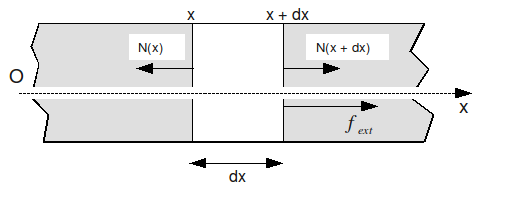
Figure 3.1.1-a : Axially loaded beam segment.

The beam has a section \(S(x)\) and is made of a material with a density \(\rho (x)\) and a Young’s modulus \(E(x)\). The fundamental principle of mechanics makes it possible to write:

\[-\ mathrm {N} (x) +\ mathrm {N} (x+\ mathit {xx}) +\ underset {x} {\ overse {x+\ mathit {xx}} {\ int}} {\ int}}} {\ int}}} {\ int}}} {\ int}}} {\ int}} {\ int}} {\ o{ x+\ mathit {xx}} {\ int}}\ rho (s)}\ rho (s) S (s)\ frac {{\ partial} ^ {2}\ mathrm {u} (s)} {\ partial {t}} ^ {2}}\ mathit {ds}}\]

where u is the displacement on the \(x\) axis of the segment

So:

\[\ frac {\ mathrm {N} (x+\ mathit {xx}) -\ mathrm {N} (x)} {\ mathit {xx}} +\ frac {1} {\ mathit {xx}}}\ underset {x}}\ underset {x}} {\ mathrm {xx}} {\ mathrm {f}}} {\ mathit {xx}}} {\ mathrm {f}}} {\ mathit {xx}}} {\ mathrm {f}}}}\ underset {x}}\ underset {x}} {\ mathrm {xx}}} {\ mathrm {f}}} {\ mathit {xx}}} {\ mathrm {f}}} {\ mathit {xx}}} m {ext}} (s)\ mathit {ds} =\ frac {1} {\ frac {1} {\ mathit {xx}}\ underset {x} {x+\ mathit {xx}} {\ int}} {\ int}}}\ rho S\ frac {1}} {\ frac {1}} {\ frac {1}} {\ frac {1} {\ partial}} {\ partial}}\ mathit {ds}}\]

Passing to the limit when \(dx\to 0\), we get:

\[\]

: label: 3.1.1-1

frac {dN (x)} {text {xx}}} + {f}} + {f} _ {text {ext}} ^ {(x)} =rho Sfrac {{partial} ^ {partial} ^ {2}} u} {partial {2}} u} {partial {2} u} {partial} u} {partial} u} {partial} u} {partial {2} u} {partial} u} {partial} u} {partial {2} u} {partial} u} {

We only keep the terms of the first order and we replace them in 3.1.1-1, then we use Hooke’s law and the hypothesis that the beam consists of longitudinal fibers working only in traction-compression to express the axial force by:

\[\]

: label:

N (x) =text {ES}frac {partial u} {partial x}

We thus obtain after simplification by \(dx\):

\[\]

: label: 3.1.1-3

frac {partial} {partial x} (text {ES}}frac {partial u} {partial x}) + {partial x}) + {f} _ {text {ext}} =rho Sfrac {{partial}} {{partial}} {partial}}

which represents the first-order local balance of a beam, for a traction-compression movement.

3.1.2. Lagrangian method

Using the beam segment in the figure, the total kinetic energy of the beam of length \(l\) is written as:

\[{E} _ {c} =\ frac {1} {2} {\ int} {2} {\ int} _ {0} ^ {l}\ rho S {\ left (\ frac {\ partial\ mathrm {u}}} {\ partial\ mathrm {u}}}} {\ partial t} {2}\ text {x}}\]

For the following, we will note the elementary kinetic energy \({E}_{{c}_{e}}=\frac{1}{2}\rho S{\left(\frac{\partial \mathrm{u}}{\partial t}\right)}^{2}\).

The internal deformation energy, thanks to Hooke’s law, is written as:

\[{E} _ {{p} _ {\ text {int}}}} =\ frac {1} {2} {\ int} _ {0} ^ {l}\ text {ES} {\ left (\ frac {\ partial\ partial\ partial\ mathrm {u}}} {\ partial x} {u}}} {\ partial x}\ right)} ^ {2}\ text {x} {\ left (\ frac {\ partial\ partial\ partial\ mathrm {u}}}} {\ partial x}\ right)} ^ {2}\ text {xx}\]

We will also note \({E}_{{p}_{{\text{int}}_{e}}}=\frac{1}{2}\text{ES}{\left(\frac{\partial \mathrm{u}}{\partial x}\right)}^{2}\).

We also have the work of the external force given by:

\[{E} _ {{p} _ {\ text {ext}}}} = {\ int} _ {o} ^ {l} {f} _ {\ text {ext}}} u\ text {ext}} u\ text {ext}}\]

and at the elementary level \({E}_{{p}_{{\text{ext}}_{e}}}={f}_{\text{ext}}\text{.}u\)

The Lagrangian is given by:

\[L= {E} _ {c} - {E} _ {{p} _ {{p} _ {\ text {int}}}} - {E} _ {{p} _ {\ text {ext}}} _ {\ text {ext}}}\]

and the Lagrangian density:

\[L= {E} _ {{c} _ {e}} - {E}} - {E}} - {E}} - {{c} _ {e}}} - {{p}} _ {{p} _ {{p} _ {p} _ {p} _ {p}} _ {e}}\]

For the continuous one-dimensional system, the Lagrange equation is written in this case:

\[\]

: label: 3.1.2-1

frac {partial L} {partial u} {partial u} -frac {partial u}}right) -frac {partial L} {partial utext {“}}right) -frac {partial}}right) -frac {partial u}}right) -frac {partial u}}right) =0

where \({u}^{'}\) and \(\dot{u}\) respectively denote the derivative with respect to \(x\) and with respect to time. Its application obviously brings us back to the equation of motion of a girder under traction-compression 3.1.1-3.

3.2. The pure twist (Saint-Venant twist)

Torsion is the rotational movement around the longitudinal axis of the beam. We assume here that the center of gravity is confused with the center of rotation (of torsion) [R3.03.03], and the warping of the section is overlooked. The case of the eccentricity of the center of torsion with respect to the center of gravity is treated in [§ 5.1].

3.2.1. Local equilibrium equation

We consider a segment of length \(dx\) rotated under the action of an internal moment \({M}_{x}\) [Figure 3.2.1-a] and an external torque \({\Gamma }_{x}\) per unit of length.

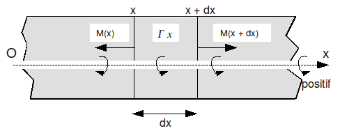
Figure 3.2.1-a : Beam segment rotating around \((\mathrm{Ox})\)

The segment is rotated by an angle \({\theta }_{x}\) with respect to the undeformed position. So we have:

3.2.1.1. Circular cross section beam

\[- {M} _ {x} (x) + {M} _ {x} (x+\ text {xx}) + {\ int} _ {x} ^ {x+\ text {xx}} {\ Gamma} _ {\ Gamma} _ {x} _ {x} (s)\ text {x} (s)\ text {ds} (s)\ text {ds} = {\ int} _ {x}} = {\ int} _ {x}} {I} _ {x}}\ frac {{\ partial} ^ {2} {\ theta} {\ theta} _ {x}} {\ partial {t} ^ {2}}}\ text {ds}}\]

with \({I}_{{q}_{x}}={\int }_{s}\rho {r}^{2}\text{ds}\) is the plane moment of inertia of section \(S\) around the axis of rotation \((\mathrm{0,}x)\).

As for traction, we obtain after division by \(\text{dx}\) and crossing the limit:

\[\ frac {d {M} _ {x}}} {\ text {xx}} {\ text {xx}}} + {\ Gamma} _ {\ theta} _ {x}}\ frac {{\ partial}}}\ frac {{\ partial}}} {{\ partial}}}\ frac {{\ partial}}}\ frac {{\ partial}}}\ frac {{\ partial}} ^ {2}} {\ partial}}\]

The law of behavior is introduced:

\[{M} _ {x} =G {I} _ {p}\ frac {\ partial {\ theta} _ {x}} {\ partial x}} {\ partial x}\]

where \(G\) is the Coulomb modulus (or shear modulus) and \({I}_{p}\) is the polar geometric moment with respect to the center of gravity of the section. (By the way, we have: \({I}_{{\theta }_{x}}=\rho {I}_{p}\) for a material with a homogeneous density).

We then get the expression:

(3.5)\[ \ frac {\ partial} {\ partial x}\ left (G {I} _ {p}\ frac {\ partial {\ theta} _ {x}} {\ partial x}\ right)\ text {+} {\ Gamma} {\ Gamma} _ {\ Gamma} _ {x}} = {I} _ {\ theta} = {I} _ {\ theta}}}\ frac {{\ partial}} ^ {2} {\ Gamma} _ {\ Gamma} _ {\ Gamma} _ {x} = {I}} = {I} _ {\ theta}}}\ frac {{\ partial}} ^ {2} {\ Gamma} {\ Gamma} _ {\ Gamma} _ {\ Gamma} _ {x}} {\ partial {t} ^ {2}}\]

which represents the first-order local equilibrium of a beam segment for a torsional movement.

3.2.1.2. Beam of any cross section

To take account of warping while remaining in the free twist hypothesis, in the case of non-circular sections, it is necessary to replace moment \({I}_{p}\) by a torsional constant \(C\) (less than \({I}_{p}\)) in the torsional equation ([R3.03.03]) in the torsional equation ([] for the calculation of \(C\)).

By definition, \({M}_{x}=GC\frac{\partial {\theta }_{x}}{\partial x}\). We then obtain:

(3.6)\[ \ frac {\ partial} {\ partial x}\ left (GC\ frac {{\ theta}} _ {\ partial x}} {\ partial x}\ right)\ text {+} {\ Gamma} _ {x} =\ rho C\ frac {{\ partial}}\ left (GC\ frac {{\ theta}} _ {\ partial x}}\ right)\ text {+} {\ Gamma} _ {x} _ {x} _ {x}} =\ rho C\ frac {{\ partial x}} =\ rho C\ frac {{\ partial}} {\ partial}}\]

When the center of gravity of the section is not the center of rotation, this expression is not valid and the torsional and flexural movements are coupled.

3.2.2. Lagrangian method

In the same way as at [§ 3.1.2], we have the kinetic energy (for example for a circular cross-section beam):

\[{E} _ {c} = {\ int} _ {0} _ {0} ^ {0} ^ {l} ^ {l}\ frac {1} {2} {I} _ {\ theta}} {\ left (\ frac {\ partial {\ theta}} _ {\ partial theta} _ {\ theta} _ {\ partial t}\ right)} ^ {2}\ text {xx}} {\ left (\ frac {\ partial {\ theta}} {\ partial {\ theta}} {\ left (\ frac {\ partial {\ theta}}\]

Internal potential energy

\[{E} _ {{p} _ {\ text {int}}}} = {\ int}}} = {\ int} _ {0} ^ {l}\ frac {1} {2} {\ mathit {GI}}} _ {p} {\ p} {\ p} {\ p} {\ p} {\ p} {\ p} {\ p} {\ p} {\ p} {\ left (\ frac {\ partial {int}}} {\ left (\ frac {\ partial {\ theta}} _ {\ partial theta} _ {\ theta} _ {x}} {\ partial t}\ right)} ^ {2}\ text {xx}\]

And the work of the outside couple

\[{E} _ {{p} _ {\ text {ext}}}} = {\ int}}} = {\ int} _ {0} ^ {l} {\ Gamma} _ {\ theta} {\ theta} _ {\ theta} _ {x} _ {x}\ text {xx}\]

By applying the Lagrange equation 3.1.2-1 to the variable \({\theta }_{x}\), we naturally end up with (3.5) giving the motion of a pure torsional beam.

3.3. Simple bending

Flexion is the translational and rotational movement around an axis perpendicular to the longitudinal axis of the beam. Here we are talking about simple bending (around \(\mathrm{Oy}\) or \(\mathrm{Oz}\)). We limit ourselves to the case of straight beams. Curved beams are treated with [§ 8].

The flexure equation is described in plane \((O,x,z)\), the extension to plane \((O,x,y)\) is immediate [Figure 3.3-a].

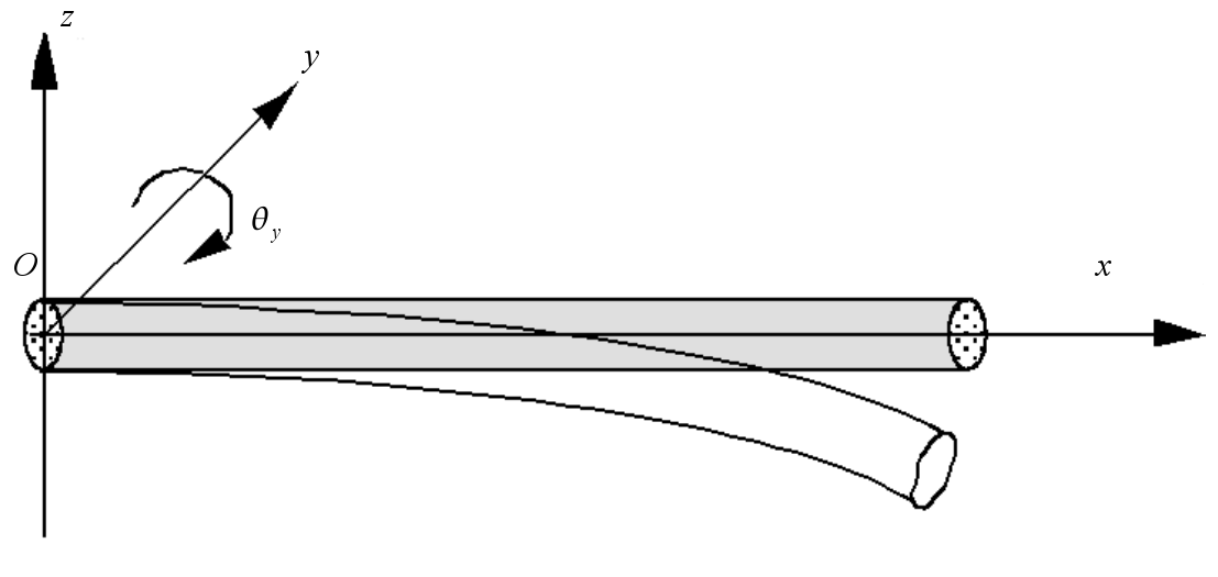
Figure 3.3-a : Bending a beam in the plane \((O,x,z)\) .

The translation along the \((O,z)\) axis is noted \(w\) and the rotation around \((O,y)\) is noted \({\theta }_{y}\).

3.3.1. Local equilibrium equation

We consider a segment of length \(\mathrm{dx}\) subjected to the shear force \({V}_{z}\), the bending moment \({M}_{y}\), an external force \({t}_{{z}_{\text{ext}}}\) distributed uniformly per unit of length, and an external torque \({m}_{{y}_{\text{ext}}}\) distributed uniformly per unit of length [Figure 3.3.1-a].

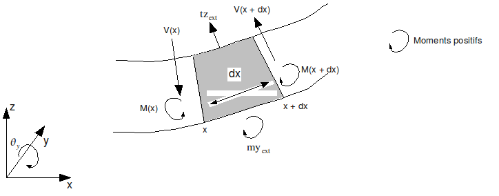
Figure 3.3.1-a : Bending beam segment in plane \((O,x,z)\)

The local balance of forces and moments (on the x-axis section \(x+\mathrm{dx}\)) gives for the forces:

\[- {V} _ {z} (x) + {V} _ {z} _ {z}\ left (x+\ text {xx}\ right) + {\ int} _ {x} ^ {x+\ text {xx}} {t}} {t}} _ {{z} _ {z} _ {z} _ {z} _ {x}}}\ rho S\ text {ds}\ frac {{\ partial} ^ {2} w} {\ partial {t} ^ {2}}}\]

And for the moments

\[- {M} _ {y} (x) + {M} _ {y}\ left (x+\ text {xx}\ right) + {\ int} _ {x} ^ {x+\ text {xx}} {m} {m}} {m}} _ {{y} _ {y} _ {y} _ {y} _ {x}} {x}} {x}} {x+\ text {xx}} {m}} {m} _ {m} _ {x}} {m} _ {m} _ {x}} {m} _ {m} _ {x}} {m} _ {m} _ {x}} {m} _ {m} _ {x}} {m}} {m} _ {m} _ {x}} {m}} {m} _ {x _ {z}\ left (x\ right)\ text {ds} = {\ int} = {\ int} = {\ int} _ {ds} = {\ text {ds}\ text {ds}\ frac {\ partial}\ frac {{\ partial}} ^ {2} ^ {2} ^ {2}} {\ theta} _ {y}} {\ partial}} {\ partial} ^ {2}}\]

We overlook the terms in \(\mathrm{dx²}\). Passing to the limit when \(\mathrm{dx}\) approaches 0, we get:

\[\begin{split}\ begin {array} {c}\ frac {\ partial {V} _ {v} _ {z}} {\ partial x}} + {\ partial x} + {{z} _ {\ text {ext}}}} =\ rho S\ frac {{\ partial} {{V}} _ {\ partial}} {\ partial}} {\ partial}} {\ partial}} {\ partial}} {\ partial}} {\ partial} w} {\ partial} w} {\ partial} w} {\ partial} w} {\ partial {2} w} {\ partial x}} {\ partial {2}}}\\ frac {\ partial {M}}} {\ partial}}} {\ partial {M}}}} {\ partial}}} - {V} _ {z} + {m} _ {{y} _ {{y} _ {\ text {ext}}}} =\ rho {I} _ {y}\ frac {{\ partial} ^ {2} {2} {\ theta}} {\ theta} _ {\ theta} _ {y}} _ {\ partial}}\ end {array}}\end{split}\]

We note that the uniformly distributed effort \({t}_{{z}_{\text{ext}}}\) produces a term that is of the second order in the balance of moments and is thus overlooked. The behavioral relationships of the resistance of the materials are then introduced.

\[\]

: label: 3.3.1-1

{M} _ {y} = EI_ {y}frac {partial {theta} _ {y}} {partial x}text {and} {V} _ {z} = {k} _ {z}\ z}\ text {z}\text {z}\\\ text {SG}left (frac {partial w}} {partial x}left)

The 3.3.1-1 expression for \({V}_{z}\) is due to Timoshenko [bib 4] where \({k}_{z}\) is the shear coefficient in the \(z\) direction. It characterizes the Timoshenko beam model; we will see later that the Euler beam model corresponds to a simplification of the Timoshenko model. \({I}_{z}\) is the geometric moment of the section with respect to the \((O,y)\) axis.

As a result, we arrive at the two equations coupled in \(w\) and \({\theta }_{y}\) for the bending in the plane \((O,x,z)\).

\[\]

: label: 3.3.1-2

frac {partial} {partial x}left [{k} _ {z}text {SG}left (frac {partial w} {partial x}} + {theta} _ {y}right)right)right)right]right]right]right]right]right]right]] + {t} _ {z} _ {z} _ {z} _ {z} _ {z} _ {text {ext}}}} =rho Sfrac {{partial x}} + {theta} _ {y}right)right)right]right]right]right] + {t} _ {z} _ {z} _ {z} _ {z} _ {z} _ {} {partial {t} ^ {2}}

\[\]

: label: 3.3.1-3

frac {partial} {partial x}left [EI_ {y}left [{y}left [{y}}frac {partial x}right] - {k} _ {z}text {SG}left (frac {partial w}left (frac {partial w}}left (frac {partial w}} {theta}}} {y}right) + {m} _ {y}right) + {m} _ {y}right) + {m} _ {y} _ {y} _ {text {ext}}} =rho {I} _ {y} _ {y}frac {{partial} ^ {2} {theta} _ {y}}} {partial {i}} {partial {t}} ^ {2}}

When the beam is uniform, that is to say that the cross section and the material are constant on the longitudinal axis, equations 3.3.1-2 and 3.3.1-3 are reduced to a single equation in \(w\). To do this, we derive the equilibrium equation of moments 3.3.1-3 only once with respect to the abscissa x.

\(EI_{y}\frac{{\partial }^{3}{\theta }_{y}}{\partial {x}^{3}}-{k}_{z}\text{SG}\left(\frac{{\partial }^{2}w}{\partial {x}^{2}}+\frac{\partial {\theta }_{y}}{\partial x}\right)=\rho {I}_{y}\frac{{\partial }^{3}{\theta }_{y}}{\partial x\partial {t}^{2}}\)

It will be observed that this manipulation eliminates the presence of the term resulting from a uniformly distributed external couple. Then, equation 3.3.1-2 can be written in the form:

\[\ frac {\ partial {\ theta} _ {y}}} {\ partial x}} =-\ frac {{\ partial} ^ {2} w} {\ partial {x} ^ {2}} -\ frac {{t}} _ {{t} _ {{z} _ {z} _ {2}}} -\ frac {{t} _ {2}}} -\ frac {{t} _ {2}}} -\ frac {{t} _ {2}}} -\ frac {{t} _ {2}}} -\ frac {{t} _ {2}}} -\ frac {{t} _ {2}}} -\ frac {{t} _ {2}}} -\ frac {{t} _ {2}}} {k} _ {z} G}\ frac {{\ partial} ^ {2} w} {\ partial {t} ^ {2}}\]

\[\]

: label: 3.3.1-4

EI_ {y}frac {{partial} ^ {4} w} {partial {4} w} {partial {x}} ^ {4}} +rho Sfrac {{partial} ^ {2} w} {partial {t}} ^ {2}}} -rho {2}} w} {partial} ^ {2} w} {partial} w} {partial} ^ {2} w} {partial {t} ^ {2}}} -rho {I}}} -rho {I} _ {y}left [1+frac {E} {{k}} _ {z} G}right] frac {{partial} ^ {4} w} {partial {x} w} {partial {x} ^ {2}} {partial}} +frac {{rho} ^ {2} {I} _ {y}}} {{y}}}} {{y}}} {{y}}} {{y}}} {{y}}} {{y}}} {{y}}} {{y}}} {{y}}} {{y}}} {{y}}} {{k}}} {{k} _ {z} G}frac {{partial} ^ {4}}} {partial} ^ {4}}} {partial} ^ {4}}} - {t} _ {4}}} - {t} {{z} _ {text {ext}}} =0

It is still useful for this type of equation to recall the physical meaning of the various terms, in order to be aware of the overlooked effects when simplifying.

\(EI_{y}\frac{{\partial }^{4}w}{\partial {x}^{4}}\) balances the loading density in the direction of translation due to the bending moment.

\(\rho S\frac{{\partial }^{2}w}{\partial {t}^{2}}\) is the translational inertia term.

\(\rho {I}_{y}\frac{{\partial }^{4}w}{\partial {x}^{2}\partial {t}^{2}}\) represents the flexural rotational inertia.

\(\rho {I}_{y}\frac{E}{{k}_{z}G}\frac{{\partial }^{4}w}{\partial {x}^{2}\partial {t}^{2}}\) is an additional term for rotational inertia due to the consideration of transverse shear (Timoshenko hypothesis).

\(\frac{{\rho }^{2}{I}_{y}}{{k}_{z}G}\frac{{\partial }^{4}w}{\partial {t}^{4}}\) results from the coupling between the rotational inertia and the translational inertia arising from the shear force.

The Timoshenko beam model (POU_D_T) takes into account all of these terms, especially those relating to shear force. It is therefore possible to model beams with low slenderness.

The Euler beam model (POU_D_E) is a simplification since shear force deformations are neglected as well as rotational inertia (it is involved in dynamic studies only for high modes). These hypotheses are justified in the case of a sufficiently large slender beam. Therefore, for the Euler model, the equation of flexural motion, in the general case of beams with variable cross section, is written:

\[\]

: label: 3.3.1-5

frac {partial} {partial {x} ^ {2}}} (EI_ {y}}frac {{partial} ^ {2} w} {partial {x} ^ {2}}) +rho Sfrac {{partial} ^ {2}}}} ({partial}}}} ({y}}}frac {partial} ^ {2} w} {partial} ^ {2} w} {partial} ^ {2}}) +rho Sfrac {frac {partial} ^ {2}}}) +rho Sfrac {{partial} ^ {2}}}) +rho Sfrac {partial} ^ {2}}}) +rho Sfrac {}} =0

Moreover, it is effectively the cutting force that causes the rotation of the straight sections with respect to the neutral axis. Neglecting this effect is like writing that \({V}_{z}=0\) leads to 3.3.1-1.

\[\]

: label: 3.3.1-6

{theta} _ {y} =-frac {partial w} {partial x}

which is the translation of Euler’s hypothesis.

For the bending in plane \((O,x,y)\), the same approach leads to [eq] for the Timoshenko beam at:

\[\]

: label: 3.3.1-7

begin {cases}

frac {partial} {partial x}left [{k} _ {y}text {SG} (frac {partial v} {partial x} - {theta} _ {z})right]right] + {t} _ {{y}} _ {{y} _ {{y} _ {y} _ {y} _ {y} _ {y} _ {y} _ {y} _ {text {ext}}}} & =rho Sfrac {{partial}} ^ {z})right] + {t} _ {{y} _ {y} _ {y} _ {y} _ {y} _ {y} _ {y} _ {y} _ {y} _ {y} _ {y} partial {t} ^ {2}}\ frac {partial} {partial x}left [EI_ {z}left [{z}}frac {partial {theta} | {z}} {partial x}right] - {k} _ {y}text {text {SG}text {SG}} (frac {partial v}}frac {partial v}frac {partial v} {partial x} _ {z}) + {{m} _ {z}text {SG}} (frac {partial v}} {partial v} {partial x} - {partial x} - {z}) + {{m} _ {z}text {SG}} (frac {partial v}} {partial v} {partial x}} ext}}} & =rho {I} _ {z} _ {z}frac {{partial} ^ {2} {theta} _ {z}}} {partial {t}} ^ {2}}

end {cases}

and when the section is constant:

\[\]

: label: 3.3.1-8

EI_ {z}frac {{partial} ^ {4} v} {partial {4}}} {partial {t} ^ {4}} -rho Sfrac {{partial} ^ {2} v} {partial {t}} ^ {2}}} -rho {2}}} -rho {I} _ {2}}} -rho {I} _ {2}} v} {partial} v} {partial {t} ^ {2}}} -rho {I} _ {2}}} -rho {I} _ {2}}} -rho {I} _ {2}}} -rho {I} _ {y} G})frac {{2} G})frac {{partial} ^ {4} v} {partial {x}} ^ {2}partial {x} ^ {2}} +frac {{rho} ^ {2} {I} _ {z}}} {{k}} {{k}} {{k}} _ {y} G}frac {{partial}} ^ {4}}} + {t}} {z}}} {{z}}} {{z}}} {{z}}} {{k}} {{k} _ {G}}frac {partial}} ^ {4}}} + {t} _ {y} _ {text {ext}}}} =0

The use of the Euler hypothesis in plane \((O,x,y)\) \({\theta }_{z}=\frac{\partial v}{\partial x}\) makes it possible to arrive at the equation of the bending motion for an Euler beam according to 3.3.1-9:

\[\]

: label: 3.3.1-9

frac {partial} {partial {x} ^ {2}}}left [EI_ {z}}frac {{partial} ^ {2} v} {partial {x} ^ {2}}right] -rho Sfrac {{partial} ^ {2}}}left [{z}}left [{z}}frac {partial} ^ {2} v} {partial} ^ {2} v} {partial} ^ {2} v} {partial} ^ {2}} v} {partial {x} ^ {2}}} {right}] -rho Sfrac {partial} ^ {2}}}right] -rho Sfrac {{partial} ^ {2}}} text {ext}}} =0

3.3.2. Lagrangian method

Kinetic energy is expressed by:

\[{E} _ {c} =\ underset {0} {\ o{ l} {\ int}}\ frac {1} {2}\ rho {I} _ {y} {(\ frac {\ partial {\ theta}} _ {\ theta} _ {\ theta} _ {\ theta} _ {\ theta} _ {\ theta} _ {\ theta} _ {\ theta} _ {\ theta} _ {\ theta} _ {\ theta} _ {\ theta} _ {\ theta} _ {\ theta} _ {\ theta} _ {\ theta} _ {\ theta} _ {theta} _ {\ theta} _ {theta} _ {theta} _ {theta} _ {theta} _ {theta} int}}\ frac {1} {2}\ rho S {(\ frac {\ partial w} {\ partial t})} ^ {2}\ text {xx}\]

according to rotational and translational movements.

Internal potential energy is equal to:

\[{E} _ {{p} _ {\ text {int}}}} = {\ int}}} = {\ int} _ {0}\ frac {1} {2}\ text {EI} {(\ frac {\ partial {\ theta}} _ {\ partial theta}} _ {\ partial theta} _ {\ partial {\ theta} _ {\ partial {\ theta} _ {\ partial {\ theta} _ {y}} _ {y}}} {y}}} {y}}} {\ partial x})} ^ {2}\ frac 1} {2}\ left [{\ iint} _ {s} {\ sigma} _ {\ sigma} _ {T}} (\ frac {\ partial w} {\ partial x}} + {\ theta} _ {y})\ text {dS}\ right]\ text {x} + {\ theta} _ {y})\ text {x}\]

where \({\sigma }_{{c}_{T}}\) is the transverse shear stress and the term \(\frac{\partial w}{\partial x}+{\theta }_{y}\) the shear strain. The Euler beam model neglects this term while the Timoshenko model hypothesizes the distribution of \({\sigma }_{{c}_{T}}\) stresses in section, consistent with the expression 3.3.1-1. In the general case of the Timoshenko model, the internal potential energy is written as:

\[{E} _ {{p} _ {\ text {int}}}} = {\ int}}} = {\ int} _ {0}\ frac {1} {2}\ text {EI} {(\ frac {\ partial {\ theta}} _ {\ partial theta}} _ {\ partial theta} _ {\ partial {\ theta} _ {\ partial {\ theta} _ {\ partial {\ theta} _ {y}} _ {y}}} {y}}} {y}}} {\ partial x})} ^ {2}\ frac 1} {2} {k} _ {z}\ text {SG} {(\ frac {\ partial w} {\ partial x} + {\ theta} _ {y})} ^ {y})} ^ {2}\ text {xx}\]

For its part, the potential for external loads is expressed by:

\[{E} _ {{p} _ {\ text {ext}}}} =- {\ text {ext}}}} =- {\ text {ext}}} {\ text {ext}}}\ text {xx} - {\ int} - {\ int} - {\ int} - {\ int} _ {0}} {0} ^ {l} {m} ^ {m} ^ {m} {m} _ {y}} _ {\ text {ext}}}} {\ theta} _ {x}}} {\ theta} _ {x}}} {\ theta} _ {y}\ text {xx}\]

The use of the Lagrange equation [eq] applied once to the variable \(w\) and then to the variable \({\theta }_{y}\) brings us back to the two equations 3.3.1-2 and 3.3.1-3 describing the flexural motion of a beam segment.