9. Loads#

The different types of loading developed for « MECA_POU_D_E « , » MECA_POU_D_T « , girder elements in linear elasticity are:

Types or options	MECA_POU_D_E	MECA_POU_D_T
CHAR_MECA_EPSI_R: loading by imposing a deformation (such as thermal stratification)	developed	developed
CHAR_MECA_PESA_R: loading due to gravity	developed	developed
CHAR_MECA_FR1D1D: loading distributed by real values	developed	expanded
CHAR_MECA_FF1D1D: loading distributed by function	developed	developed
CHAR_MECA_TEMP_R: “thermal” loading	developed	developed
CHAR_MECA_FRELEC: “electric force” load created by a right secondary conductor	developed	developed
CHAR_MECA_FRLAPL: “electric force” load created by any secondary conductor	developed	developed

9.1. Deformation loading#

OPTION: « CHAR_MECA_EPSI_R »

The load is calculated from a state of deformation (this option was developed to take into account thermal stratification in pipes). The deformation is given by the user using the PRE_EPSI keyword in AFFE_CHAR_MECA.

The model only takes into account traction-compression and pure flexure work (no shear force, no torsional moment).

The following behavioral relationships are used:

\(N=\mathrm{ES}\frac{\partial u}{\partial x},{M}_{y}=E{I}_{y}\frac{\partial {\theta }_{y}}{\partial x},{M}_{z}=E{I}_{z}\frac{\partial {\theta }_{z}}{\partial x}\)

Thus, the second elementary member associated with this load is obtained:

at point 1: \({F}_{{x}_{1}}=E{S}_{1}\frac{\partial u}{\partial x},{M}_{{y}_{1}}=E{I}_{{y}_{1}}\frac{\partial {\theta }_{y}}{\partial x},{M}_{{z}_{1}}=E{I}_{{z}_{1}}\frac{\partial {\theta }_{z}}{\partial x}\)
at point 2: \({F}_{{x}_{2}}=E{S}_{2}\frac{\partial u}{\partial x},{M}_{{y}_{2}}=E{I}_{{y}_{2}}\frac{\partial {\theta }_{y}}{\partial x},{M}_{{z}_{2}}=E{I}_{{z}_{2}}\frac{\partial {\theta }_{z}}{\partial x}\)

By giving yourself \(\frac{\partial u}{\partial x}\text{,}\frac{\partial {\theta }_{y}}{\partial x}\) and \(\frac{\partial {\theta }_{z}}{\partial x}\) for a beam, you can assign a loading to it.

9.2. Loading due to gravity#

OPTION: « CHAR_MECA_PESA_R »

The force of gravity is given by the acceleration module \(g\) and a normed vector indicating the direction \(n\).

The principle for distributing the load over the two nodes of the beam is to take into account the \(\xi (x)\) shape functions associated with each degree of freedom of the element [§ 4]. We therefore have for a loading in gravity an equivalent nodal force \(\overrightarrow{Q}\):

\(\overrightarrow{Q}={\int }_{0}^{L}\xi (x)\rho Sg\overrightarrow{n}\text{dx}\)

Notes:

The form functions used are (simplifying hypothesis) those of the Euler-Bernoulli model.

You must, of course, place yourself in the local coordinate system of the beam to do this calculation.

Axial force (in \(x\) ):

\(\begin{array}{}{F}_{{x}_{i}}={\int }_{0}^{L}{\xi }_{i}\rho S\text{}g\cdot x\text{dx}\\ ({\xi }_{1}=1-\frac{x}{L}\text{,}{\xi }_{2}=\frac{x}{L})\end{array}\)

from where: \({F}_{{x}_{1}}=\rho g\cdot xL(\frac{{S}_{1}}{3}+\frac{{S}_{2}}{6})\) to point 1,

\({F}_{{x}_{2}}=\rho g\cdot xL(\frac{{S}_{1}}{6}+\frac{{S}_{2}}{3})\) in point 2,

for a linearly varying cross section \((S={S}_{1}+({S}_{2}-{S}_{1})\frac{x}{L})\)

and \(\begin{array}{}{F}_{{x}_{1}}=\rho g\cdot xL(\frac{3{S}_{1}+2\sqrt{{S}_{1}{S}_{2}}+{S}_{2}}{\text{12}})\text{,}\\ {F}_{{x}_{2}}=\rho g\cdot xL(\frac{{S}_{2}+2\sqrt{{S}_{1}{S}_{2}}+3{S}_{2}}{\text{12}})\end{array}\)

for a homothetically varying section \((S{\left[\sqrt{{S}_{1}}+(\sqrt{{S}_{2}-\sqrt{{S}_{1}}})\frac{x}{L}\right]}^{2})\)

Torsional moment:

Without taking warpage into account, it does not exist.

In plan \((xoz)\):

\(\begin{array}{}{F}_{{z}_{1}}=\rho g\cdot z{\int }_{0}^{L}{\xi }_{1}S\text{dx}\\ {M}_{{y}_{1}}=\rho g\cdot z{\int }_{0}^{L}{\xi }_{2}S\text{dx}\\ {F}_{{z}_{2}}=\rho g\cdot z{\int }_{0}^{L}{\xi }_{3}S\text{dx}\\ {M}_{{y}_{2}}=\rho g\cdot z{\int }_{0}^{L}{\xi }_{4}S\text{dx}\end{array}\)

\(\begin{array}{}{\xi }_{1}=2{(\frac{x}{L})}^{3}-3{(\frac{x}{L})}^{2}+1\text{,}{\xi }_{2}=L\left[-{(\frac{x}{L})}^{3}+2{(\frac{x}{L})}^{2}-\frac{x}{L}\right]\text{,}\\ {\xi }_{3}=-2{(\frac{x}{L})}^{3}+3{(\frac{x}{L})}^{2}\text{,}{\xi }_{4}=L\left[-{(\frac{x}{L})}^{3}+{(\frac{x}{L})}^{2}\right]\end{array}\)

Hence, for a cross-section varying linearly:

\(\begin{array}{}{F}_{{y}_{1}}=\rho g\cdot yL(\frac{7{S}_{1}}{20}+\frac{3{S}_{2}}{20}),{M}_{{z}_{1}}=\rho g\cdot y{L}^{2}(\frac{{S}_{1}}{20}+\frac{{S}_{2}}{30})\\ {F}_{{y}_{2}}=\rho g\cdot yL(\frac{3{S}_{1}}{20}+\frac{7{S}_{2}}{20}),{M}_{{z}_{2}}=-\rho g\cdot y{L}^{2}(\frac{{S}_{1}}{30}+\frac{{S}_{2}}{20})\end{array}\)

and, for a homothetically varying section:

\(\begin{array}{}{F}_{{z}_{1}}=\rho g\cdot zL(\frac{8{S}_{1}+5\sqrt{{S}_{1}{S}_{2}}+2{S}_{2}}{30}),{M}_{{y}_{1}}=\rho g\cdot z{L}^{2}(\frac{-2{S}_{1}-2\sqrt{{S}_{1}{S}_{2}}-{S}_{2}}{60})\\ {F}_{{z}_{2}}=\rho g\cdot zL(\frac{2{S}_{1}+5\sqrt{{S}_{1}{S}_{2}}+8{S}_{2}}{30}),{M}_{{y}_{2}}=\rho g\cdot z{L}^{2}(\frac{{S}_{1}+2\sqrt{{S}_{1}{S}_{2}}+{\mathrm{2S}}_{2}}{60})\end{array}\)

In plan \((xoy)\):

\(\begin{array}{}{F}_{{y}_{1}}=\rho g\cdot y{\int }_{o}^{L}{\xi }_{1}S\mathrm{dx},{M}_{{z}_{1}}=\rho g\cdot y{\int }_{o}^{L}-{\xi }_{2}S\mathrm{dx}\\ {F}_{{y}_{2}}=\rho g\cdot y{\int }_{o}^{L}{\xi }_{3}S\mathrm{dx},{M}_{{z}_{2}}=\rho g\cdot y{\int }_{o}^{L}-{\xi }_{4}S\mathrm{dx}\end{array}\)

Hence, for a cross-section varying linearly:

and, for a homothetically varying section:

\(\begin{array}{}{F}_{{y}_{1}}=\rho g\cdot yL(\frac{8{S}_{1}+5\sqrt{{S}_{1}{S}_{2}}+2{S}_{2}}{30}),{M}_{{z}_{1}}=\rho g\cdot y{L}^{2}(\frac{2{S}_{1}+2\sqrt{{S}_{1}{S}_{2}}+{S}_{2}}{60})\\ {F}_{{y}_{2}}=\rho g\cdot yL(\frac{2{S}_{1}+5\sqrt{{S}_{1}{S}_{2}}+8{S}_{2}}{30}),{M}_{{z}_{2}}=\rho g\cdot y{L}^{2}(\frac{-{S}_{1}-2\sqrt{{S}_{1}{S}_{2}}-2{S}_{2}}{60})\end{array}\)

9.3. Distributed loads#

OPTIONS: « CHAR_MECA_FR1D1D « , » CHAR_MECA_FF1D1D « ,

Loads are given under the FORCE_POUTRE keyword, either by real values in AFFE_CHAR_MECA (option CHAR_MECA_FR1D1D), or by functions in AFFE_CHAR_MECA (option CHAR_MECA_FF1D1D).

The various possibilities are:

	constant load	loading varying linearly
straight beam with constant cross section	developed	developed
straight beam with linearly varying cross section	developed	no
straight beam with homothetically varying cross section	developed	no

For straight beams with a constant cross section, the distributed load is composed of forces and moments that are constant or that vary linearly along the axis of the beam. In all other cases, the distributed load is only composed of constant force.

The method used to calculate the load to be imposed on the nodes is that presented in [§ 4.1.2].

9.3.1. Straight beam with constant cross section#

For a loading that is constant or linearly varying, we obtain:

\({F}_{{x}_{1}}\mathrm{=}L(\frac{{n}_{1}}{3}+\frac{{n}_{2}}{6}),{F}_{{x}_{2}}\mathrm{=}L(\frac{{n}_{1}}{6}+\frac{{n}_{2}}{3}),{M}_{{x}_{1}}\mathrm{=}L(\frac{{m}_{{t}_{1}}}{3}+\frac{{m}_{{t}_{2}}}{6}),{M}_{{x}_{2}}\mathrm{=}L(\frac{{m}_{{t}_{1}}}{6}+\frac{{m}_{{t}_{2}}}{3})\)

\({n}_{1}\) and \({n}_{2}\) are the components of the axial loading at points 1 and 2, \({m}_{{t}_{1}}\) and \({m}_{{t}_{2}}\) are the components of the torsional moment at points 1 and 2, derived from user data placed in the local coordinate system.

\({t}_{{y}_{1}}\), \({t}_{{y}_{2}}\), \({t}_{{z}_{1}}\) and \({t}_{{z}_{2}}\) are the components of the shear force, \({m}_{{y}_{1}}\), \({m}_{{y}_{2}}\), \({m}_{{z}_{1}}\) and \({m}_{{z}_{2}}\) are the components of the bending moments, at points 1 and 2, from the user data placed in the local coordinate system.

\(\begin{array}{cc}{F}_{{y}_{1}}\mathrm{=}L(\frac{7{t}_{{y}_{1}}}{20}+\frac{3{t}_{{y}_{2}}}{20})\mathrm{-}\frac{({m}_{{z}_{1}}+{m}_{{z}_{2}})}{2}& {M}_{{y}_{1}}\mathrm{=}\mathrm{-}{L}^{2}(\frac{{t}_{{z}_{1}}}{20}+\frac{{t}_{{z}_{2}}}{30})\mathrm{-}\frac{({m}_{{y}_{2}}\mathrm{-}{m}_{{y}_{1}})L}{12}\\ {F}_{{y}_{2}}\mathrm{=}L(\frac{3{t}_{{y}_{1}}}{20}+\frac{7{t}_{{y}_{2}}}{20})+\frac{({m}_{{z}_{1}}+{m}_{{z}_{2}})}{2}& {M}_{{y}_{2}}\mathrm{=}{L}^{2}(\frac{{t}_{{z}_{1}}}{30}+\frac{{t}_{{z}_{2}}}{20})+\frac{({m}_{{y}_{2}}\mathrm{-}{m}_{{y}_{1}})L}{12}\\ {F}_{{z}_{1}}\mathrm{=}L(\frac{7{t}_{{z}_{1}}}{20}+\frac{3{t}_{{z}_{2}}}{20})+\frac{({m}_{{y}_{1}}+{m}_{{y}_{2}})}{2}& {M}_{{z}_{1}}\mathrm{=}{L}^{2}(\frac{{t}_{{y}_{1}}}{20}+\frac{{t}_{{y}_{2}}}{30})\mathrm{-}\frac{({m}_{{z}_{2}}\mathrm{-}{m}_{{z}_{1}})L}{12}\\ {F}_{{z}_{2}}\mathrm{=}L(\frac{3{t}_{{z}_{1}}}{20}+\frac{7{t}_{{z}_{2}}}{20})\mathrm{-}\frac{({m}_{{y}_{1}}+{m}_{{y}_{2}})}{2}& {M}_{{z}_{2}}\mathrm{=}\mathrm{-}{L}^{2}(\frac{{t}_{{y}_{1}}}{30}+\frac{{t}_{{y}_{2}}}{20})+\frac{({m}_{{z}_{2}}\mathrm{-}{m}_{{z}_{1}})L}{12}\end{array}\)

9.3.2. Straight beams with variable cross section#

The load provided must be constant. A method similar to that used by self-weight is used [§ 55].

The load provided should be constant along the element. The load reduced to the nodes is equivalent to that which can be obtained by using the results of [§ 9.3.1]. With a constant load, it becomes:

\(\begin{array}{cccc}{F}_{{x}_{1}}=L\frac{n}{2}& {F}_{{x}_{2}}=L\frac{n}{2}& {F}_{{y}_{1}}=L\frac{{t}_{y}}{2}& {F}_{{y}_{2}}=L\frac{{t}_{y}}{2}\\ {M}_{{z}_{1}}={L}^{2}\frac{{t}_{y}}{12}& {M}_{{z}_{2}}=-{L}^{2}\frac{{t}_{y}}{12}& {F}_{{z}_{1}}=L\frac{{t}_{z}}{2}& {F}_{{z}_{2}}=L\frac{{t}_{z}}{2}\\ {M}_{{y}_{1}}=-{L}^{2}\frac{{t}_{z}}{12}& {M}_{{y}_{2}}={L}^{2}\frac{{t}_{z}}{12}& & \end{array}\)

9.4. Thermal charging#

OPTION: « CHAR_MECA_TEMP_R »

To obtain this load, it is necessary to calculate the deformation induced by the temperature difference \(T-{T}_{\text{référence}}\):

\(\begin{array}{}{u}_{1}=-L\alpha (T-{T}_{\text{référence}})\\ {u}_{2}=L\alpha (T-{T}_{\text{référence}})\end{array}\) (\(\alpha\): thermal expansion coefficient)

Then, we calculate the induced forces: \(F=Ku\). Since \(K\) is the stiffness matrix local to the element, a base change must then be made to obtain the values of the load components in the global coordinate system.

9.5. Electric charging#

OPTIONS: « FORCE_ELEC « , » INTE_ELEC ».

This type of load makes it possible to take into account the Laplace force acting on a main conductor, due to the presence of a secondary conductor.

Secondary conductor \(«\mathrm{2 }»\) is straight and does not rely on part of the Aster mesh if the « FORCE_ELEC » option is used.

The secondary conductor is not necessarily straight and can rely on part of the Aster mesh if the « INTE_ELEC » option is used.

The linear density of the Laplace force exerted at a point \(M\) of the main conductor by the secondary conductor is written:

\(f(M)=\frac{1}{2}{e}_{1}\wedge {\int }_{2}\frac{{e}_{2}\wedge r}{{\parallel r\parallel }^{3}}\mathrm{ds}\) with \({\parallel {e}_{1}\parallel }^{2}={\parallel {e}_{2}\parallel }^{2}=1\)

Note:

To obtain the Laplace force, the vector returned as a result of the calculation performed by one of these two options must be multiplied by the intensity time function specified by the « DEFI_FONC_ELEC « operator. [U4.MK.10]

9.5.1. Finite or infinite right secondary conductor#

OPTION: « FORCE_ELEC » [U4.44.01]

For a finite secondary conductor, we have:

\(\overrightarrow{f}(M)=\frac{{e}_{1}}{2}\wedge \frac{n}{d}(\mathrm{sin}{\alpha }_{1}-\mathrm{sin}{\alpha }_{2})\)

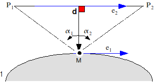
with \(\begin{array}{}n=\frac{{e}_{2}\wedge d}{d}\\ d=∥d∥\end{array}\)

For an infinite secondary conductor, we have:

\(f(M)={e}_{1}\wedge \frac{n}{d}\)

Three types of loading are possible:

infinite parallel right conductor,
multiple infinite parallel straight conductors,
right conductor in any finite or infinite position.

For the case of an infinite parallel right conductor, its position can be given in two ways:

or by a translation vector from the main conductor to the secondary conductor,
or by the distance between the two conductors and by a point on the secondary conductor.

A constant loading on the entire main element is therefore obtained. We can thus use the technique presented in [§ 9.3] [§ 9.4] to calculate the loading at the nodes.

\(\begin{array}{c}{\mathrm{F}}_{1}=\mathrm{f}(M)\frac{L}{2},{\mathrm{F}}_{2}=\mathrm{f}(M)\frac{L}{2},{\mathrm{M}}_{1}={\mathrm{e}}_{1}\wedge \mathrm{f}(M)\frac{{L}^{2}}{12},{\mathrm{M}}_{2}=-{\mathrm{e}}_{1}\wedge \mathrm{f}(M)\frac{{L}^{2}}{12}\\ \mathrm{f}(M)=\mathit{cste}\forall M\end{array}\)

For the case of multiple infinite parallel straight conductors, we must directly give the standardized « Laplace force » vector. Since this is usually given in the global coordinate system, it is necessary to determine the « Laplace force » vector in the local coordinate system of the main element. Thus, in the same way as before, the loading at the nodes is calculated.

For the case of a right conductor in any finite or infinite position, its position is given by two points \({P}_{1}\) and \({P}_{2}\) such that the current flows from \({P}_{1}\) to \({P}_{2}\). The load does not have to be constant along the main element.

The method chosen to calculate the reduced load at the nodes is obviously the same as before. But here, the integration is done numerically by discretizing the element into a certain number (in practice: 100 points between \({P}_{1}\) and \({P}_{2}\)).

Thus, we integrate:

\(\begin{array}{}{F}_{1}={\int }_{0}^{L}f(M)\text{}\left[2{(\frac{x}{L})}^{3}-3{(\frac{x}{L})}^{2}+1\right]\text{dx}\\ {F}_{2}={\int }_{0}^{L}f(M)\text{}\left[-2{(\frac{x}{L})}^{3}+3{(\frac{x}{L})}^{2}\right]\text{dx}\end{array}\)

\(\begin{array}{}{\overrightarrow{M}}_{1}={\int }_{0}^{L}-{\overrightarrow{e}}_{1}\wedge \overrightarrow{f}(M)\left[L(-{(\frac{x}{L})}^{3}+2{(\frac{x}{L})}^{2}-\frac{x}{L})\right]\text{dx}\\ {\overrightarrow{M}}_{2}={\int }_{0}^{L}-{\overrightarrow{e}}_{1}\wedge \overrightarrow{f}(M)\left[L(-{(\frac{x}{L})}^{3}+{(\frac{x}{L})}^{2})\right]\text{dx}\end{array}\)

Note:

Like \(f(M)\cdot x\text{=}0\) and \(({e}_{1}\wedge f(M))\cdot x=0,(x\text{=}{e}_{1})\)

only the shape functions associated with the flexure problem are used.

9.5.2. Secondary conductor described by a part of mesh ASTER#

OPTION: « INTE_ELEC « , [U4.44.01]

The secondary driver as a whole is not necessarily straight. But it is described only by straight elements. Its length is necessarily finite.

Its position can be completed by the use of a translation vector or a plane symmetry (by a point and a normal vector normalized by the plane of symmetry) with respect to the main conductor.

Apart from the fact that it is necessary to sum up the interaction of the various elements of the secondary conductor on the main conductor, the method is the same as before (case \((\mathrm{iii})\)).

**Note:**For digital integration, 5 points between *:math:`{P}_{1}`*and:math:`{P}_{2}`* are used only 5 points between * and .