7. E modeling#
7.1. Characteristics of modeling#
The load is of the tensile — pure compression type.
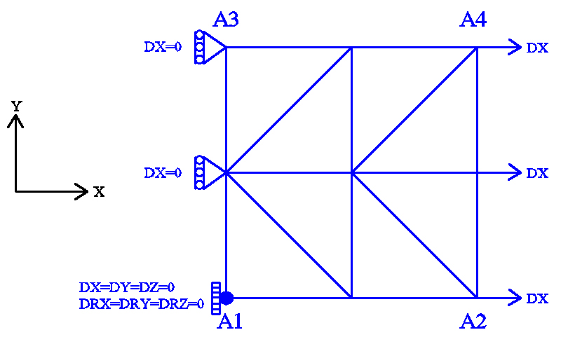
Figure 7.1-a : mesh and boundary conditions.
Modeling: DKTG
Boundary conditions:
Embedding in \({A}_{1}\);
\(\mathrm{DX}=0.0\) on the \({A}_{1}-{A}_{3}\) edge;
\(\mathrm{DX}={U}_{0}\times f(t)\) on the \({A}_{2}-{A}_{4}\) edge;
where \({U}_{0}=1.0\times {10}^{-3}m\) and \(f(t)\) represent the amplitude of cyclic loading as a function of the (pseudo-time) parameter \(t\). To properly verify the model, we consider a loading function as follows:
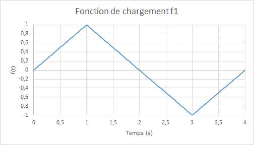
Figure 7.1-b : loading function: traction, then compression
Note: the extreme deformation is: \(1.0\times {10}^{-3}\) , or about a third of the deformation during the transition to plasticity of steels. No integration time: \(0.025\) .
7.2. Characteristics of the mesh#
Number of knots: 9.
Number of stitches: 8 TRIA3; 8 SEG2.
7.3. Tested sizes and results#
We compare the reaction forces along the \(\mathit{Ox}\) axis in \(\mathit{A1}\mathrm{-}\mathit{A3}\) and the displacements along the \(\mathit{Oy}\) en \(\mathit{A4}\) axis obtained by the multilayer modeling with the ENDO_ISOT_BETON law and by that based on the BETON_REGLE_PR law, in terms of relative differences; the tolerances are taken in absolute value:
Identification |
Reference type |
Reference value |
Tolerance |
|
TRACTION - ELASTIQUE \(t=\mathrm{0,25}\) |
||||
Relative difference \(\mathit{FX}\) |
|
1 10-6 |
||
Relative difference \(\mathrm{DY}\) |
|
1 10-6 |
||
TRACTION - ENDOMMAGEMENT \(t=\mathrm{1,0}\) |
||||
Relative difference \(\mathrm{FX}\) |
|
1 10-6 |
||
TRACTION - DECHARGEMENT \(t=\mathrm{1,5}\) |
||||
Relative difference \(\mathrm{FX}\) |
|
1 10-6 |
||
COMPRESSION - CHARGEMENT \(t=\mathrm{2,5}\) |
||||
Relative difference \(\mathrm{FX}\) |
|
1 10-6 |
||
COMPRESSION - DECHARGEMENT \(t=\mathrm{3,5}\) |
||||
Relative difference \(\mathrm{FX}\) |
|
1 10-6 |
||
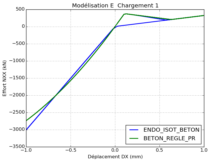
Comparative effort graphs \({N}_{\mathrm{xx}}\) — displacement \(\mathrm{DX}\) **in****traction —****compression for load:math:`f`**: :
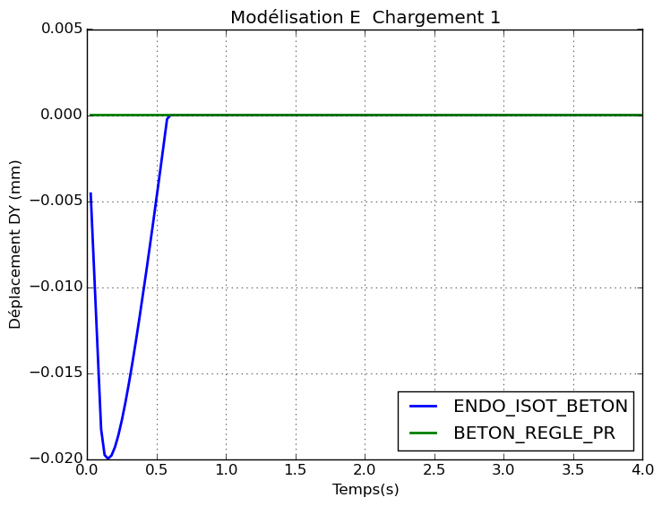
Comparative graphs displacement \(\mathrm{DY}\) (due to the Poisson effect) as a function of time:
7.4. notes#
The test case carried out here aims to test model BETON_REGLE_PRsous stresses that are significant enough for steels to effectively recover their stiffness.
The behavior is similar in traction for laws BETON_REGLE_PRet ENDO_ISOT_BETON under load: the differences appear for a significant compression due to the parabolic response of law BETON_REGLE_PR. In traction, after the concrete ruins, we find the stiffness corresponding to the resumption of forces by the steel.
The landfill response is not taken into account by law BETON_REGLE_PR (elastic response)
The deformation due to the Poisson effect is not taken into account by law BETON_REGLE_PR. For law ENDO_ISOT_BETON, DY displacements are not zero before the appearance of concrete ruins around 0.1 s.
Since the convergence of the model with law BETON_REGLE_PRest is difficult around time 0.6s (stiffness recovery) with the matrix TANGENTE, the matrix ELASTIQUE is then used.