6. D modeling#
6.1. Characteristics of modeling#
The load is of the distortion and pure shear type in the plane.
|
|
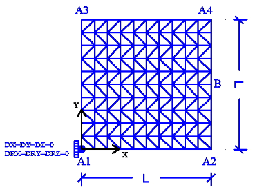
Figure 6.1-a : m**mesh and boundary conditions**
Modeling: DKT. \(L=1.0m\).
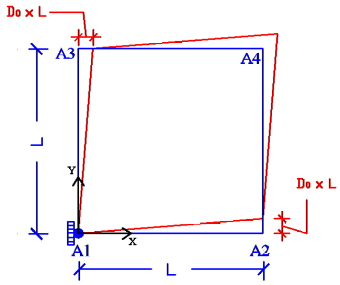
Boundary conditions (see figure above on the right) so that the plate is subject to pure distortion: \({\varepsilon }_{\text{xy}}\) must be constant or to pure shear so forces are applied. Therefore, the following displacement field is applied to the edges of the plate for distortion:
\(\mathrm{\{}\begin{array}{c}{u}_{x}\mathrm{=}{D}_{0}\mathrm{\cdot }y\\ {u}_{y}\mathrm{=}{D}_{0}\mathrm{\cdot }x\end{array}\mathrm{\Rightarrow }{\varepsilon }_{\mathit{xy}}\mathrm{=}\frac{1}{2}({u}_{x,y}+{u}_{y,x})\mathrm{=}{D}_{0}\)
So:
we impose an embedding in \({A}_{1}\),
\({u}_{x}={D}_{0}\cdot y,{u}_{y}=0\) on edge \({A}_{1}-{A}_{3}\), \({u}_{x}=0,{u}_{y}={D}_{0}\cdot x\) on edge \({A}_{1}-{A}_{2}\),
\({u}_{x}={D}_{0}\cdot y,{u}_{y}={D}_{0}\cdot L\) on edge \({A}_{2}-{A}_{4}\), \({u}_{x}={D}_{0}\cdot L,{u}_{y}={D}_{0}\cdot x\) on edge \({A}_{3}-{A}_{4}\),
where \({D}_{0}=3.3{10}^{-4}\) and \(f(t)\) represent the magnitude of cyclic loading as a function of the (pseudo-time) parameter \(t\), defined as:
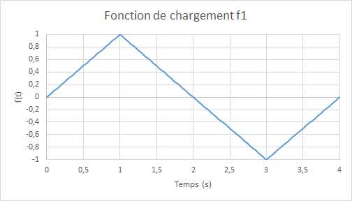
Figure 6.1-b : loading function
Integration increment: \(0.05s\).
6.2. Characteristics of the mesh#
Knots: 121.
Stitches: 200 TRIA3; 40 SEG2.
6.3. Tested sizes and results#
For the distortion, the shear force \({N}_{\mathrm{xy}}\) and \(B\) obtained by the two models are compared; the tolerances are taken in absolute values based on these relative differences:
Identification |
Reference type |
Reference value |
Tolerance |
|
DIST. POS . - PHASE CHAR. ELAS. \(t=\mathrm{0,25}\) |
||||
Relative difference in efforts \({N}_{\mathrm{xy}}\) |
|
0 |
2 10-1 |
|
DIST. POS. - PHASE CHAR. ENDO . \(t=\mathrm{1,0}\) |
||||
Relative difference in efforts \({N}_{\mathrm{xy}}\) |
|
0 |
1 10-1 |
|
DIST. POS. - PHASE**** DECHAR. ELAS .** \(t=\mathrm{1,5}\) |
||||
Relative difference in efforts \({N}_{\mathrm{xy}}\) |
|
0 |
4 10-1 |
|
DIST. NEG. - PHASE CHAR. ELAS . \(t=\mathrm{3,0}\) |
||||
Relative difference in efforts \({N}_{\mathrm{xy}}\) |
|
0 |
1 10-1 |
|
DIST. NEG. - PHASE DECHAR. ELAS . \(t=\mathrm{3,5}\) |
||||
Relative difference in efforts \({N}_{\mathrm{xy}}\) |
|
0 |
4 10-1 |
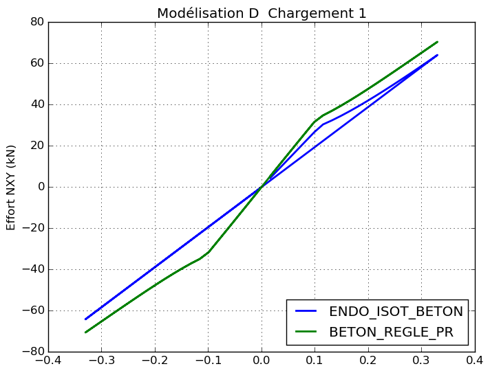
Shearing force diagram \({N}_{\mathrm{xy}}\) (in the plan) as a function of time:
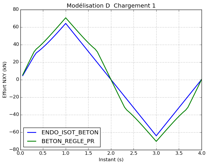
shear force graph \({N}_{\mathit{xy}}\) **** (in the plan) **based on:math:`{D}_{0}`**imposed: **
6.4. notes#
A similar shear behavior is observed for laws BETON_REGLE_PRet ENDO_ISOT_BETON under load: the shear stiffness is however higher for law BETON_REGLE_PR (~ 15%).
The landfill response is not taken into account by law BETON_REGLE_PR (elastic response).
The shear response for BETON_REGLE_PRest symmetric unlike the ENDO_BETON_ISOT law for which the memory of cracking in one direction is retained.