1. Reference problem

1.1. Geometry

The structure is a healthy square in which three interfaces are introduced, shown in red in Figure 1.1-a. The first is oblique and cuts off the entire domain. The second is vertical. It connects to the first one. The third is horizontal. It connects to the second one. The dimensions of the structure as well as the position of the interfaces are given in Figure 1.1-a and are expressed in meters, \(\text{[m]}\).

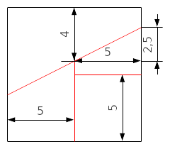
Figure 1.1-a: Geometry of the structure and positioning of the interfaces.

1.2. Material properties

The material has an isotropic elastic behavior defined by the following material parameters:

Young’s module: \(100\text{MPa}\)

Poisson’s ratio: \(0.3\)

1.3. Boundary conditions and loads

In the non-contact case (models A to D), moving conditions are applied on the left and right edges of the structure, so that each of the 4 zones has a different displacement from the others according to \(\text{X}\). This load is shown in FIG. 1.3-a. We block the movements in \(\text{Y}\) (and in \(\text{Z}\) for 3D models) on these same edges.

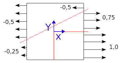
Figure 1.3-a: Illustration of boundary conditions and loads, non-contact cases.

In the case of contact (E to H models), roller conditions are imposed on the left and bottom edges and homogeneous pressure is applied on the right and top edges of \(\text{1 MPa}\). This load is represented in FIG. 1.3-b. Each block is then compressed uniformly according to \(X\) and \(Y\).

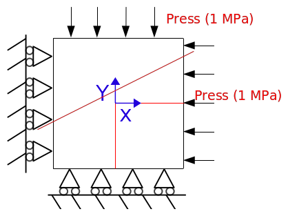
Figure 1.3-b: Illustration of boundary conditions and loads, contact cases.