3. Modeling A

3.1. Characteristics of modeling

This is a \(\text{X-FEM}\) model, in plane deformations (D_ PLAN). Interfaces are defined by level functions (normal level sets noted \(\text{LN}\)).

The equations of the level functions for the oblique, horizontal, and vertical interfaces are as follows:

\(\text{LN}1\mathrm{=}Y\mathrm{-}1\mathrm{-}\frac{X}{2}\) eq 3.1-1

\(\text{LN}2\mathrm{=}Y\) eq 3.1-2

\(\text{LN}3\mathrm{=}X\) eq 3.1-3

The oblique interface is defined in the classical way using the DEFI_FISS_XFEM operator with the normal level set \(\text{LN1}\). To define the vertical interface, we call the operator DEFI_FISS_XFEM with the normal level set \(\text{LN2}\), by defining a branch with the oblique crack via the keyword JONCTION, and by choosing a point « below » the oblique interface in the operand POINT. This step makes it possible to define crack 2 in the area below the first one (see figure 3.1-a in the center).

To define the horizontal interface, we call the operator DEFI_FISS_XFEM with the normal level set \(\text{LN3}\), by defining a branch with the vertical crack via the keyword JONCTION, and by choosing a point « to the right » in the operand POINT. This step makes it possible to define crack 3 in the area to the right of the second crack (see Figure 3.1-a on the right).

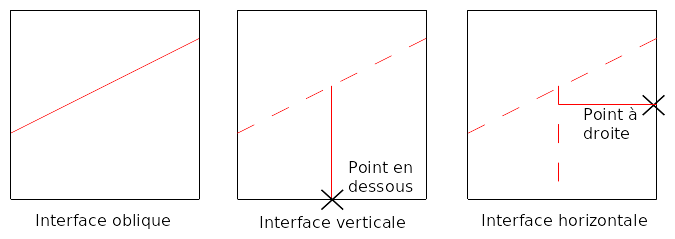
Figure 3.1-a: Intersection construction steps.

3.2. Characteristics of the mesh

The mesh, which comprises 25 cells of the QUAD4 type, is represented in FIG. 3.2-a.

It can be seen in this figure that the central mesh is cut by the three interfaces. This test therefore makes it possible to validate multiple division. The nodes in this mesh are enriched 3 times: they therefore have the degrees of freedom DX, DY, H1X, H1Y, H2X, H2Y, H3X and H3Y.

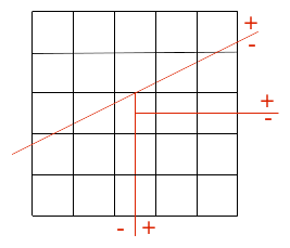
Figure 3.2-a: The modeling mesh A.

The advantage of this test is to verify that the addition of 3 discontinuity functions to the standard form function for each node of the central mesh makes it possible to represent the kinematics of movement of the 4 domains generated by the two branches (see Figure 3.2-b).

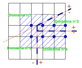
Figure 3.2-b: multi-heaviside nodes and discontinuity domains represented.

3.3. Features tested

We test the DEFI_FISS_XFEM operator with the use of the JONCTION keyword, which makes it possible to define crack branches in \(\text{X-FEM}\). The operator MODI_MODELE_XFEM is also tested in the case of meshes that are cut by several cracks. The Multi-Heaviside and the multi-storage of Data Structures (\(\text{SD}\)) \(\text{X-FEM}\) is of course activated. The assignment of Heaviside functions is verified in the integration sub-elements of the horizontal crack support (in blue in Figure 3.2-b).

We test the assembly of Heavisid degrees of freedom at the level of the matrices and the second members of the elements connected to the intersection for option COMPORTEMENT in STAT_NON_LINE.

Post-processing \(\text{X-FEM}\) is also validated in the case of multi-slicing, with the operators POST_MAIL_XFEM and POST_CHAM_XFEM.

3.4. Tested sizes and results

The movements at the level of the crack lips are tested after having carried out the post-treatment operations relating to \(\text{X-FEM}\) (POST_MAIL_XFEM and POST_CHAM_XFEM). The displacement DX must correspond to the load imposed in Figure 1.3-a on each of the zones and DY must be zero. The minimum and maximum values are tested on the lips of each zone.

Identification		Reference	% tolerance	1.00E-11
DEPZON_1	DX	MIN	-0.25
		MAX	-0.25	1.00E-11
	DY	MIN	0	1.00E-11
		MAX	0	1.00E-11
DEPZON_2	DX	MIN	-0.5	1.00E-11
		MAX	-0.5	1.00E-11
	DY	MIN	0	1.00E-11
		MAX	0	1.00E-11
DEPZON_3	DX	MIN	0.75	1.00E-11
		MAX	0.75	1.00E-11
	DY	MIN	0	1.00E-11
		MAX	0	1.00E-11
DEPZON_4	DX	MIN	0.75	1.00E-11
		MAX	0.75	1.00E-11
	DY	MIN	0	1.00E-11
		MAX	0	1.00E-11

Table 3.4-1

The deformation is shown in Figure 3.4-a. The color code represents the movement field.

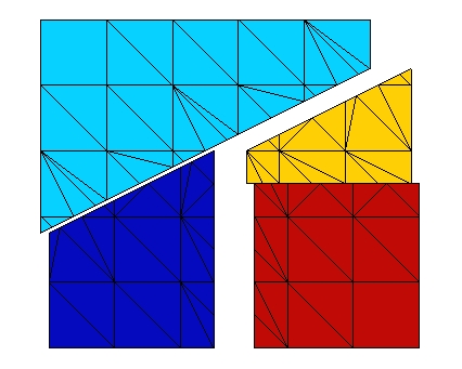
Figure 3.4-a: Deformed structure.

3.5. notes

Very good results are obtained for this test, the error recorded corresponding to the numerical residue.