6. E modeling

This modeling is based on B modeling.

The type of element chosen for the mesh is the only difference between these two models.

6.1. Characteristics of the mesh

Each HEXA8 mesh in B modeling is broken down into 6 TETRA4 for E modeling.

Thus the structure is discretized into 30 finite elements TETRA4.

The nodes on either side of the interface are enriched nodes, so the tetrahedra contained in the three central cells of modeling B that have such nodes are also enriched. Only the tetrahedra contained in the two extreme hexahedra of the B model are conventional meshes with only classical knots.

It is therefore possible to impose boundary conditions on the extreme meshes in the usual way.

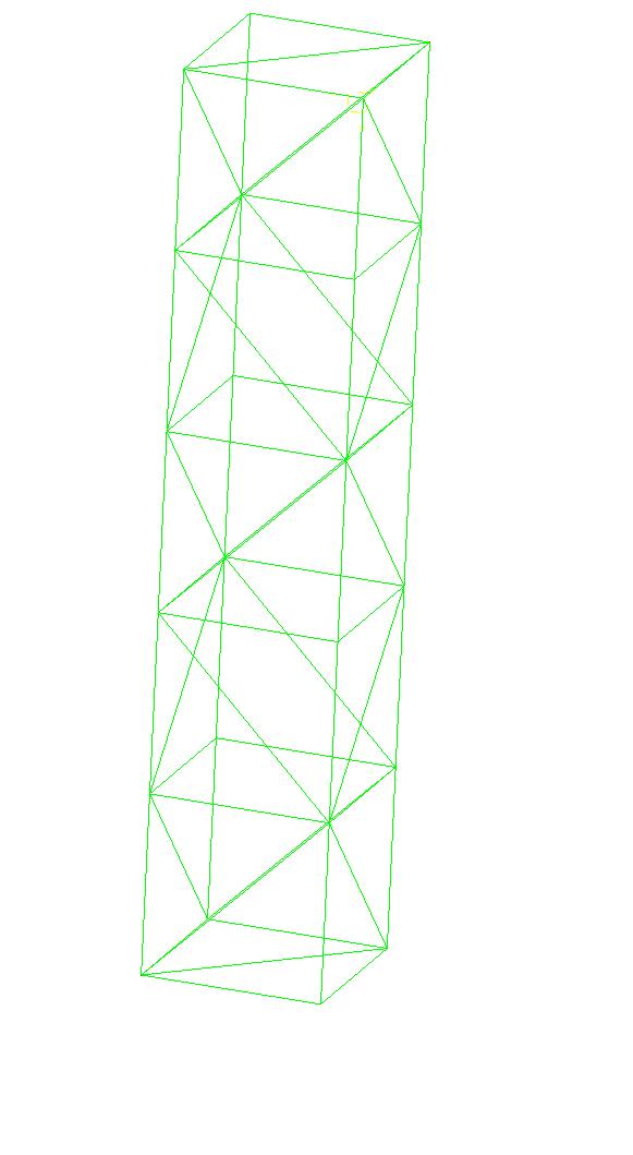
Figure 6.1-a : Mesh

6.2. Boundary conditions

The nodes on the lower face are embedded and the nodes on the upper face are forced to move:

Lower side: \(\mathrm{DX}=0\), \(\mathrm{DY}=0\), and \(\mathrm{DZ}=0\)

Upper side: \(\mathrm{DX}=0\), \(\mathrm{DY}=0\) and \(\mathrm{DZ}=\mathrm{uz}\) .

This is the first loading case.

In fact, we take the freedom to move the upper part of the structure in the three directions, so we will choose as the 2nd load case:

Lower side: \(\mathrm{DX}=0\), \(\mathrm{DY}=0\), and \(\mathrm{DZ}=0\)

Upper side: \(\mathrm{DX}=\mathrm{ux}\), \(\mathrm{DY}=\mathrm{uy}\) and \(\mathrm{DZ}=\mathrm{uz}\)

\(\mathrm{ux}={10}^{-6}\)

\(\mathrm{uy}=2.{10}^{-6}\)

\(\mathrm{uz}=3.{10}^{-6}\)

6.3. Analytical resolution

The solution of such a problem is of course still obvious: all the movements following \(x\) and \(y\) are zero, all the movements following \(z\) below the level set are zero and all the movements following \(z\) above the level set are equal to the displacement imposed \({u}_{z}\) at the top of the structure.

6.4. Tested sizes and results

The displacement values are tested after convergence of the iterations of the operator STAT_NON_LINE. We check that we find the values determined in [§ 3.3] for the 2 load cases.

The following table is obtained for the first loading case.

Identification	Reference	Tolerance
\(\mathit{DX}\) for all nodes just below the interface	0.00	1.0E-16
\(\mathit{DY}\) for all nodes just below the interface	0.00	1.0E-16
\(\mathit{DZ}\) for all nodes just below the interface	0.00	1.0E-16
\(\mathit{DX}\) for all nodes just above the interface	0.00	1.0E-16
\(\mathit{DY}\) for all nodes just above the interface	0.00	1.0E-16
\(\mathit{DZ}\) for all nodes just above the interface	1.0E-6	1.0E -9%

The following table is obtained for the 2nd load case.

Identification	Reference	Tolerance
\(\mathit{DX}\) for all nodes just below the interface	0.00	1.0E-16
\(\mathit{DY}\) for all nodes just below the interface	0.00	1.0E-16
\(\mathit{DZ}\) for all nodes just below the interface	0.00	1.0E-16
\(\mathit{DX}\) for all nodes just above the interface	1.0E-6	1.0E -9%
\(\mathit{DY}\) for all nodes just above the interface	2.0E-6	1.0E -9%
\(\mathit{DZ}\) for all nodes just above the interface	3.0E-6	1.0E -9%

To test all the nodes at once, we test the MINIMUM and the MAXIMUM of the column.

6.5. Comments

We notice the discontinuity of the field of movement when crossing the interface, which is possible thanks to the enrichment of the elements with the Heaviside degree of freedom.