2. Modeling A

2.1. Characteristics of the mesh

The structure is meshed by a single HEXA8 mesh. The interface is therefore present within this element through level sets.

2.2. Boundary conditions

Recall that the displacement under X- FEM is the sum of a continuous displacement and a discontinuous displacement. In the case of an interface, with no cracks, the approximation of the displacement is written as follows:

\({u}^{h}(x)=\sum _{i\in {N}_{n}(x)}{a}_{i}{\varphi }_{i}(x)+\sum _{j\in {N}_{n}(x)\cap {K}_{\text{+}}}{b}_{j}{\varphi }_{j}(x)\left(\text{-2}{\chi }_{\text{-}}\left(\mathit{lsn}(x)\right)\right)+\sum _{j\in {N}_{n}(x)\cap {K}_{\text{-}}}{b}_{j}{\varphi }_{j}(x)\left(\text{2}{\chi }_{\text{+}}\left(\mathit{lsn}(x)\right)\right)\)

Where:

\({a}_{i}\) and \({b}_{i}\) are the degrees of freedom of movement at node \(i\),

\({\phi }_{i}\) the shape functions associated with node \(i\),

\({N}_{n}(x)\) is the set of nodes whose support contains the point \(x\),

\({K}_{\text{-}}\) is the set of nodes located in domain \(\mathit{lsn}(x)<0\), and whose support is entirely cut by the interface,

\({K}_{\text{+}}\) is the set of nodes located in domain \(\mathit{lsn}(x)>0\), and whose support is entirely cut by the interface,

\({\chi }_{\text{-}}(x)\) is a domain characteristic function defined by \({\chi }_{\text{-}}(x)=\{\begin{array}{c}1\text{si}x<0\\ 0\text{si}x\ge 0\end{array}\),

\({\chi }_{\text{+}}(x)\) is a domain characteristic function defined by \({\chi }_{\text{+}}(x)=\{\begin{array}{c}0\text{si}x<0\\ 1\text{si}x\ge 0\end{array}\),

\(\mathit{lsn}(x)\) is the normal level-set value at point \(x\)

For more details, refer to the reference documentation X- FEM [R7.02.12].

Since the nodes near the interface, i.e. here the 8 nodes of the mesh, are enriched by additional degrees of freedom, the boundary conditions are written a bit differently. This relates to the enrichment of classical form functions [R7.02.12] by the characteristic functions of domains \({\chi }_{\text{-}}(x)\) and \({\chi }_{\text{+}}(x)\).

Imposing zero displacement on the nodes on the underside is the same as writing a linear relationship between the degrees of freedom. For each node, we impose \({a}_{\mathit{ix}}=0\) (same as following \(y\) and \(z\)) when the interface does not conform to the nodes of the mesh. However, if the interface was in accordance with the nodes, imposing zero displacement on the interface also underlies a hypothesis with respect to the jump in movement through the interface. This introduces an additional relationship due to the continuity/jump of movement. It is then appropriate to impose the following condition on the degrees of freedom of discontinuity \({\mathrm{2b}}_{\mathit{ix}}=\Delta u=0\).

For the nodes on the upper face, we impose a following displacement \(z\) equal to \({10}^{-6}\) and zero in the other two directions, that is to say \({a}_{\mathit{ix}}=0\), \({a}_{\mathit{iy}}=0\) and \({a}_{\mathit{iz}}={10}^{-6}\).

These relationships are automated when using the DDL_IMPO keyword on an X- FEM node. For example, the imposition of the following \(X\) null displacement of the node X- FEM \(\mathit{N1}\) is therefore done in the classical way:

DDL_IMPO =_F (NOEUD =”N1”, DX=0)

2.3. Analytical resolution

The solution to such a problem is, of course, obvious. It can be seen that mechanically speaking, the two parts of the structure will detach: the lower part will have zero displacement and the upper part will have an overall movement equal to the imposed displacement (see []).

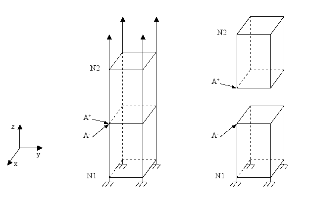
Figure 2.3-a : Initial and final states of the structure

The analytical solution is then as follows: all the movements following \(x\) and \(y\) are zero, all the movements following \(z\) below the level set are zero and all the movements following \(z\) above the level set are equal to the imposed displacement \({u}_{z}\) at the top of the structure.

2.4. Tested sizes and results

The POST_MAIL_XFEM operator makes it possible to mesh the cracks represented by the X- FEM method. The POST_CHAM_XFEM operator then makes it possible to export the X- FEM results to this new mesh. These two operators should only be used after the calculation in post-processing views. They allow nodes to be generated just below and above the interface and to show their movements.

We therefore test the values of the displacement just below and above the interface after convergence of the iterations of the operator STAT_NON_LINE. We check that we find the values determined in [§ 2.3].

Identification	Reference	Tolerance
\(\mathit{DX}\) for all nodes just below the interface	0.00	1.0E-16
\(\mathit{DY}\) for all nodes just below the interface	0.00	1.0E-16
\(\mathit{DZ}\) for all nodes just below the interface	0.00	1.0E-16
\(\mathit{DX}\) for all nodes just above the interface	0.00	1.0E-16
\(\mathit{DY}\) for all nodes just above the interface	0.00	1.0E-16
\(\mathit{DZ}\) for all nodes just above the interface	1.0E-6	1.0E -9%

To test all the nodes at once, we test the MINIMUM and the MAXIMUM of the column.

2.5. Comments

We notice the discontinuity of the field of movement when crossing the interface, which is possible thanks to the enrichment of the elements with the Heaviside degree of freedom.