3. B modeling

3.1. Characteristics of the mesh

The structure is discretized into 5 cells of the HEXA8 type.

The nodes on either side of the interface are enriched nodes, so the three central cells with such nodes are also enriched. Only the two extreme stitches are classic knits with only classic knots.

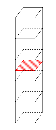
Figure 3.1-a : mesh with 5 HEXA8

3.2. Boundary conditions

The boundary conditions applied represent the same physical phenomenon as for modeling A. The nodes on the lower face are embedded and a displacement of the nodes on the upper face is imposed:

Underside (Knots \(\mathrm{N1}\), \(\mathrm{N6}\), \(\mathrm{N11}\), \(\mathrm{N16}\)): \(\mathrm{DX}=0\), \(\mathrm{DY}=0\), and \(\mathrm{DZ}=0\)

Upper side (Knots \(\mathrm{N21}\), \(\mathrm{N22}\), \(\mathrm{N23}\), \(\mathrm{N24}\)): \(\mathrm{DX}=0\), \(\mathrm{DY}=0\), and \(\mathrm{DZ}=\mathrm{uz}\)

This is the first loading case.

In fact, we take the freedom to move the upper part of the structure in the three directions, so we will choose as the 2nd load case:

Underside (Knots \(\mathrm{N1}\), \(\mathrm{N6}\), \(\mathrm{N11}\), \(\mathrm{N16}\)): \(\mathrm{DX}=0\), \(\mathrm{DY}=0\), and \(\mathrm{DZ}=0\)

Top side: \(\mathrm{DX}=\mathrm{ux}\), \(\mathrm{DY}=\mathrm{uy}\), and \(\mathrm{DZ}=\mathrm{uz}\)

\(\mathrm{ux}={1.10}^{-6}\)

\(\mathrm{uy}=2.{10}^{-6}\)

\(\mathrm{uz}=3.{10}^{-6}\)

3.3. Analytical resolution

The solution to such a problem is, of course, still obvious. All the movements following \(x\) and \(y\) are zero, all the movements following \(x\), \(y\) and \(z\) below the level set are zero and all the movements following \(x\), \(y\) and \(z\) above the level set are equal to the imposed displacement \({u}_{x}\), \({u}_{y}\) and \({u}_{z}\) at the top of the structure.

3.4. Tested sizes and results

The displacement values are tested after convergence of the iterations of the operator STAT_NON_LINE. We check that we find the values determined in [§ 3.3] for the 2 load cases.

The following table is obtained for the first loading case.

Identification	Reference	Tolerance
\(\mathit{DX}\) for all nodes just below the interface	0.00	1.0E-16
\(\mathit{DY}\) for all nodes just below the interface	0.00	1.0E-16
\(\mathit{DZ}\) for all nodes just below the interface	0.00	1.0E-16
\(\mathit{DX}\) for all nodes just above the interface	0.00	1.0E-16
\(\mathit{DY}\) for all nodes just above the interface	0.00	1.0E-16
\(\mathit{DZ}\) for all nodes just above the interface	1.0E-6	1.0E -9%

The following table is obtained for the 2nd load case.

Identification	Reference	Tolerance
\(\mathit{DX}\) for all nodes just below the interface	0.00	1.0E-16
\(\mathit{DY}\) for all nodes just below the interface	0.00	1.0E-16
\(\mathit{DZ}\) for all nodes just below the interface	0.00	1.0E-16
\(\mathit{DX}\) for all nodes just above the interface	1.0E-6	1.0E -9%
\(\mathit{DY}\) for all nodes just above the interface	2.0E-6	1.0E -9%
\(\mathit{DZ}\) for all nodes just above the interface	3.0E-6	1.0E -9%

To test all the nodes at once, we test the MINIMUM and the MAXIMUM of the column.

3.5. Comments

We notice the discontinuity of the field of movement when crossing the interface, which is possible thanks to the enrichment of the elements with the Heaviside degree of freedom.