5. D modeling

This modeling is based on modeling A.

The type of element chosen for the mesh is the only difference between these two models.

5.1. Characteristics of the mesh

We discretize the structure into 6 finite elements TETRA4

The interface is present within these 6 elements through the level sets.

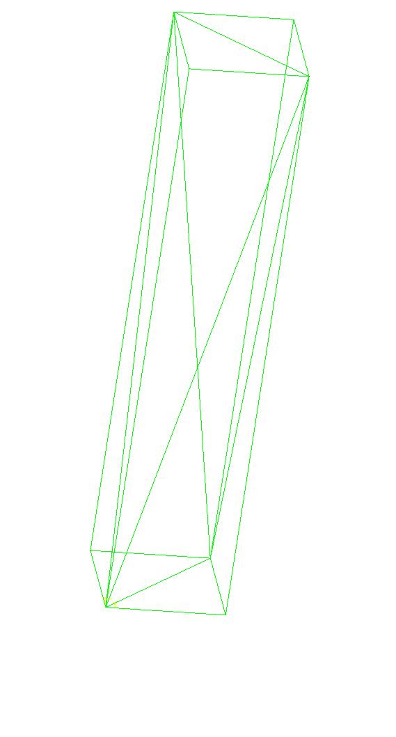
Figure 5.1-a : Mesh

5.2. Boundary conditions

The boundary conditions are those of modeling A: we embed the nodes on the lower face and we impose a displacement of the nodes on the upper face.

5.3. Analytical resolution

The analytical solution is the one presented in modeling A [§ 2.3]: all the degrees of freedom following \(x\) and \(y\) are zero and all the degrees of freedom following \(z\) are equal to \(\mathrm{uz}/2\), where \(\mathrm{uz}={10}^{-6}\)

5.4. Tested sizes and results

We test the values of the displacement just below and above the interface after convergence of the iterations of the operator STAT_NON_LINE. We check that we find the values determined in [§ 2.3].

Identification	Reference	Tolerance
DX for all nodes just below the interface	0.00	1.0E-16
DY for all nodes just below the interface	0.00	1.0E-16
DZ for all nodes just below the interface	0.00	1.0E-16
DX for all nodes just above the interface	0.00	1.0E-16
DY for all nodes just above the interface	0.00	1.0E-16
DZ for all nodes just above the interface	1.0E-6	1.0E -9%

To test all the nodes at once, we test the MINIMUM and the MAXIMUM of the column.

5.5. Comments

We notice the discontinuity of the field of movement when crossing the interface, which is possible thanks to the enrichment of the elements with the Heaviside degree of freedom.