9. K modeling#
9.1. Characteristics of modeling#
The modeling is 3D, only the edge of the frame is represented. Two calculations are performed with different pairing options, contact algorithms, and linear solvers.
9.2. Characteristics of the mesh#
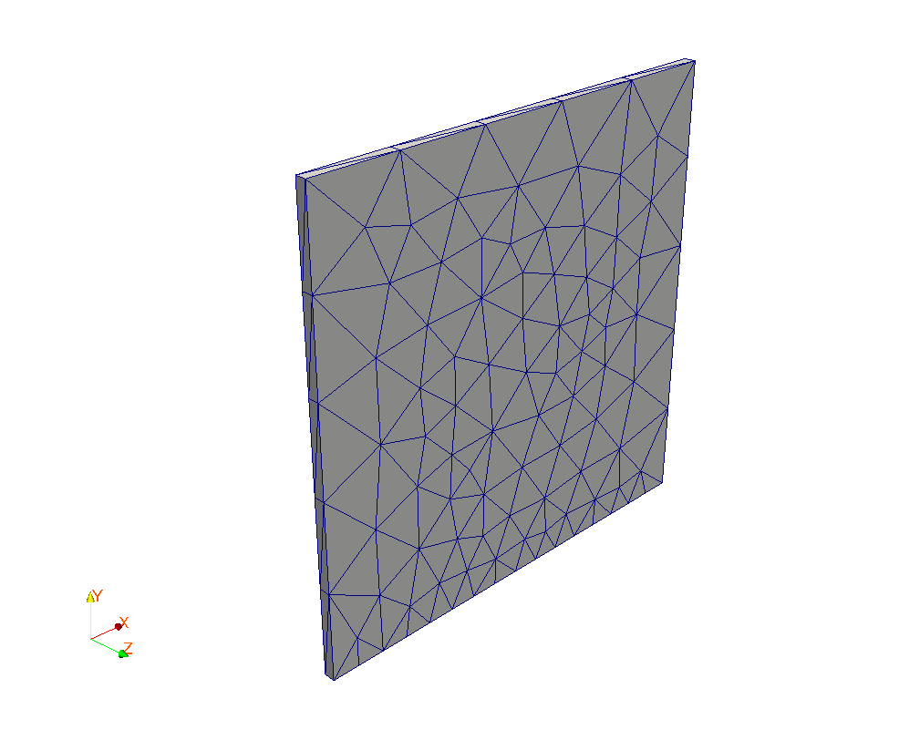
Number of knots: 1236
Number of meshes and types: 526 TETRA10 for the plate and 32 TRIA6 for the frame.
9.3. Tested sizes and results#
First calculation (controlled geometric update, node matching, algorithm “PENALISATION”, solver “MULT_FRONT”)
Identification |
Reference type |
Reference value |
Tolerance |
\(\mathit{DX}\) at the point \(A\) instant \(1.0\) |
“SOURCE_EXTERNE” |
2.86E-5 |
5.0% |
\(\mathit{DX}\) at the point \(C\) instant \(1.0\) |
“SOURCE_EXTERNE” |
2.28E-5 |
5.0% |
Second calculation (controlled geometric updating, nodal matching, algorithm “PENALISATION”, solver “LDLT”)
Identification |
Reference type |
Reference value |
Tolerance |
\(\mathit{DX}\) at the point \(A\) instant \(1.0\) |
“SOURCE_EXTERNE” |
2.86E-5 |
5.0% |
\(\mathit{DX}\) at the point \(C\) instant \(1.0\) |
“SOURCE_EXTERNE” |
2.28E-5 |
5.0% |
9.4. notes#
The results obtained in this unstructured quadratic 3D modeling are close to the reference.
The difference with the previous models is a higher penalty coefficient (high friction penalty coefficient ahead of \(a\ast E\)).
The 3D problem gives results identical to 2D following the blocking of the degrees of freedom following \(\mathit{DZ}\).