8. G modeling#
8.1. Characteristics of modeling#
The modeling is 3D, only the edge of the frame is represented. Two calculations are performed with different pairing options, contact algorithms, and linear solvers.
8.2. Characteristics of the mesh#
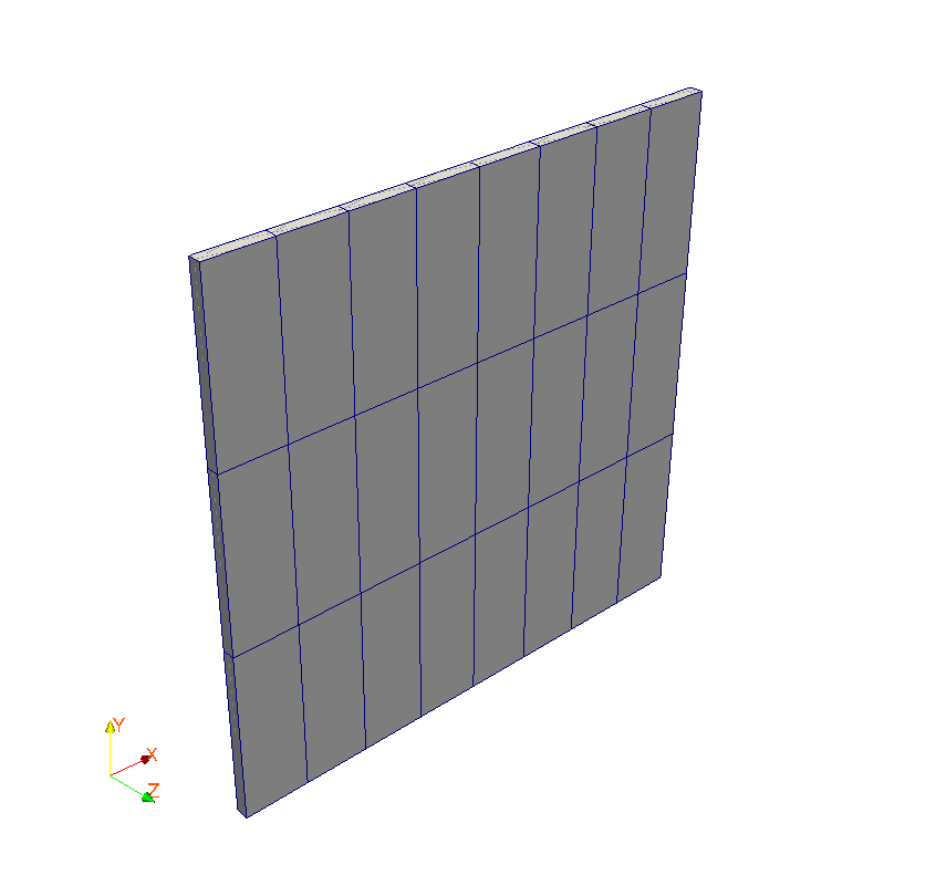
Number of knots: 408
Number of meshes and types: 24 HEXA27 for the plate and 8 QUAD9 for the frame.
8.3. Tested sizes and results#
First calculation (controlled geometric update, nodal matching, slave normal, algorithm “PENALISATION”, solver “MULT_FRONT”)
Identification |
Reference type |
Reference value |
Tolerance |
\(\mathit{DX}\) at the point \(A\) instant \(1.0\) |
“SOURCE_EXTERNE” |
2.86E-5 |
5.0% |
\(\mathit{DX}\) at the point \(C\) instant \(1.0\) |
“SOURCE_EXTERNE” |
2.28E-5 |
5.0% |
Second calculation (controlled geometric update, nodal matching, slave normal, algorithm “PENALISATION”, solver “LDLT”)
Identification |
Reference type |
Reference value |
Tolerance |
\(\mathit{DX}\) at the point \(A\) instant \(1.0\) |
“SOURCE_EXTERNE” |
2.86E-5 |
5.0% |
\(\mathit{DX}\) at the point \(C\) instant \(1.0\) |
“SOURCE_EXTERNE” |
2.28E-5 |
5.0% |
8.4. notes#
The results obtained in this quadratic 3D modeling are closer to the reference than the previous modeling due to the use of QUAD9 meshes on the contact edge.
The difference with the previous models is a higher penalty coefficient (high friction penalty coefficient ahead of \(a\ast E\)).
The 3D problem gives results identical to 2D following the blocking of the degrees of freedom following \(\mathit{DZ}\).