3. Modeling A

3.1. Characteristics of modeling

The modeling is D_ PLAN, only the edge of the frame is represented. Two calculations are performed with different linear solvers.

3.2. Characteristics of the mesh

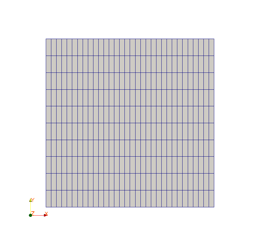
Number of knots: 396

Number of meshes and types: 320 QUAD4 for the plate and 32 SEG2 for the frame.

3.3. Tested sizes and results

First calculation (master-slave normal, controlled geometric update, algorithm “PENALISATION”, solver “MULT_FRONT”)

Identification	Reference type	Reference value	Tolerance
\(\mathit{DX}\) at the point \(A\) instant \(1.0\)	“SOURCE_EXTERNE”	2.86E-5	5.0%
\(\mathit{DX}\) at point \(B\) instant \(1.0\)	“SOURCE_EXTERNE”	2.72E-5	5.0%
\(\mathit{DX}\) at the point \(C\) instant \(1.0\)	“SOURCE_EXTERNE”	2.28E-5	5.0%
\(\mathit{DX}\) at point \(D\) instant \(1.0\)	“SOURCE_EXTERNE”	1.98E-5	5.0%
\(\mathit{DX}\) at the point \(E\) instant \(1.0\)	“SOURCE_EXTERNE”	1,5E-5	5,0%

Second calculation (master-slave normal, controlled geometric update, algorithm “PENALISATION”, solver “LDLT”)

Identification	Reference type	Reference value	Tolerance
\(\mathit{DX}\) at the point \(A\) instant \(1.0\)	“SOURCE_EXTERNE”	2.86E-5	5.0%
\(\mathit{DX}\) at point \(B\) instant \(1.0\)	“SOURCE_EXTERNE”	2.72E-5	5.0%
\(\mathit{DX}\) at the point \(C\) instant \(1.0\)	“SOURCE_EXTERNE”	2.28E-5	5.0%
\(\mathit{DX}\) at point \(D\) instant \(1.0\)	“SOURCE_EXTERNE”	1.98E-5	5.0%
\(\mathit{DX}\) at the point \(E\) instant \(1.0\)	“SOURCE_EXTERNE”	1,5E-5	5,0%

We also test the projection by considering the penultimate slave node on the right.

Identification	Reference type	Reference value	Tolerance
PROJ_Xde CONT_NOEU instant \(1.0\)	“ANALYTIQUE”	3.88E-002	1.0E-6%
PROJ_Yde CONT_NOEU instant \(1.0\)	“ANALYTIQUE”	0.00E+000	1.0E-6%

3.4. notes

The results obtained are close to the external source to within 5% (code mean). The linear solver has no influence on the results.