6. D modeling#
6.1. Characteristics of modeling#
In this modeling, the crack is meshed with Zcracks (case FEM). The mesh is free.
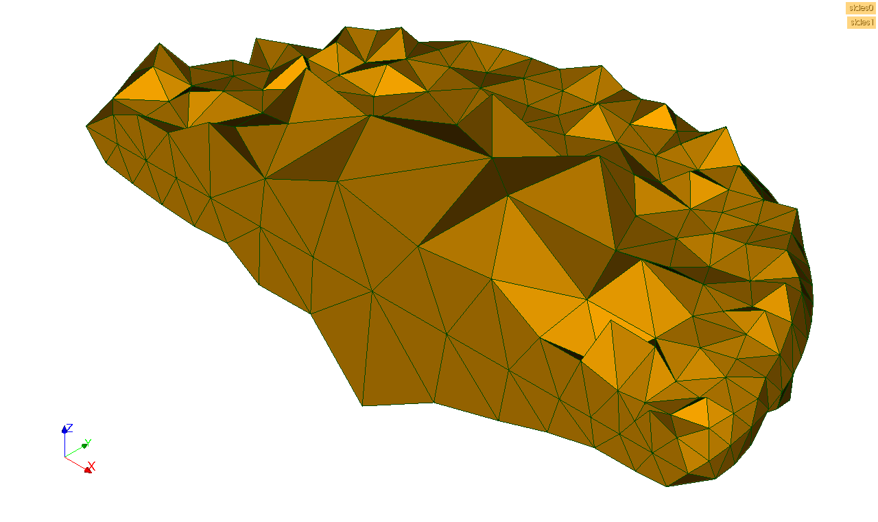
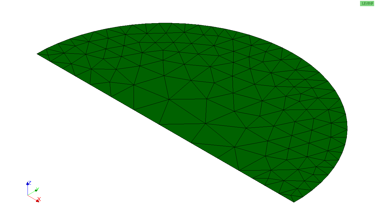
Figure 6.1-1: free mesh
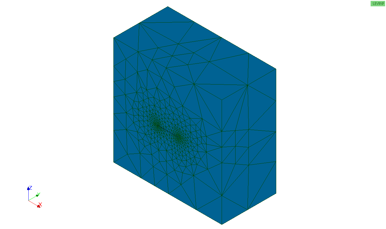
Figure 6.1-2: Structure mesh
6.2. Characteristics of the mesh#
Number of knots: 19666
Number of meshes and type: 13697 TETRA10
Number of knots at the bottom of a crack: 83
The characteristic length of an element near the crack bottom is \(\mathrm{0,15}m\).
The middle nodes of the edges of the elements touching the bottom of the crack are moved to a quarter of these edges.
6.3. Tested sizes and results#
The theta field integration crowns for command CALC_G are:
\(\text{RINF}=\mathrm{0,06}m\) and \(\text{RSUP}=\mathrm{0,22}m\).
Three types of smoothing are chosen:
LEGENDREavec DEGRE =5 (by default)
LINEAIREavec a reduced number of points at the bottom of the crack (NB_POINT_FOND = 21)
LINEAIREavec the « hat » smoothing applied afterwards
To test the value of \({K}_{I}\) for all points at the bottom of the crack, we test the \(\mathit{min}\) and the \(\mathit{max}\) values along the bottom.
\({K}_{\mathit{II}}\) is tested only to the point where \(\omega \mathrm{=}0°\) (where \({K}_{\mathit{II}}\) is normally maximum).
\({K}_{\mathit{III}}\) is tested only to the point where \(\omega \mathrm{=}90°\) (where \({K}_{\mathit{III}}\) is normally maximum).
Theoretically, you should test the absolute value of \({K}_{\mathit{II}}\) and \({K}_{\mathit{III}}\) because the sign is arbitrary.
6.3.1. Values from CALC_G option K with Legendre smoothing#
The values are in \(\mathit{Pa}\mathrm{.}\sqrt{m}\).
Identification |
Reference Type |
Reference Value |
% Tolerance |
|
\(\mathit{max}({K}_{I})\) |
“ANALYTIQUE” |
7,978 105 |
10, 0% |
|
\(\mathit{min}({K}_{I})\) |
“ANALYTIQUE” |
7,978 105 |
10, 0% |
|
\({K}_{\mathit{II}}\) in \(\omega \mathrm{=}0°\) |
“ANALYTIQUE” |
9,386 105 |
10, 0% |
|
\({K}_{\mathit{III}}\) in \(\omega \mathrm{=}90°\) |
“ANALYTIQUE” |
6,570 105 |
10, 0% |
Values from CALC_G option K with a smoothing of LINEAIRE and a reduced number of points at the bottom of the crack ~~~~~~~~~~~~~~~~~~~~~~~~~~~~~~~~~~~~~~~~~~~~~~~~~~~~~~~~~~~~~~~~~~~~~~~~~~~~~~~~~~~~~~~~~~~~~~~~~~~~~~~~~~~~~~~~~~~~~~~~~~~~~~~~~~~~~~~~~~~~~~~~~~~~~~~~~~~~~~~~~~~~~~~~~~~~~~~~~~~~~~~~~~~~~~~ ~~~~~~~~~~~~~~~~
The values are in \(\mathit{Pa}\mathrm{.}\sqrt{m}\).
Identification |
Reference Type |
Reference Value |
% Tolerance |
|
\(\mathit{max}({K}_{I})\) |
“ANALYTIQUE” |
7,978 105 |
10, 0% |
|
\(\mathit{min}({K}_{I})\) |
“ANALYTIQUE” |
7,978 105 |
10, 0% |
|
\({K}_{\mathit{II}}\) in \(\mathrm{\omega }=0°\) |
“ANALYTIQUE” |
9,386 105 |
10, 0% |
|
\({K}_{\mathit{III}}\) in \(\mathrm{\omega }=90°\) |
“ANALYTIQUE” |
6,570 105 |
10, 0% |
6.3.2. Values from CALC_G option K with a smoothing of LINEAIRE and the smoothing « hat »#
The values are in \(\mathit{Pa}\mathrm{.}\sqrt{m}\).
Identification |
Reference Type |
Reference Value |
% Tolerance |
|
\(\widehat{G}\) in \(\omega \mathrm{=}0°\) |
“ANALYTIQUE” |
6, 906 |
|
|
\(\widehat{G}\) in \(\mathrm{\omega }=90°\) |
“ANALYTIQUE” |
5,703 |
6, 0% |
|
\(\widehat{{K}_{I}}\) in \(\omega \mathrm{=}0°\) |
“ANALYTIQUE” |
7,978 105 |
11, 0% |
|
\(\widehat{{K}_{I}}\) in \(\mathrm{\omega }=90°\) |
“ANALYTIQUE” |
7,978 105 |
7,978 105 |
7,5% |
6.4. notes#
The tolerances are quite high with the use of a smoothing of LINEAIRE and NB_POINT_FOND, however, refining the mesh improves the results.
The,, and show the evolution of \(G\), \({K}_{I}\),, \({K}_{\mathit{II}}\), and \({K}_{\mathit{III}}\) along the crack background. It can be seen that the K3 is not correct. This is due to local base incorrections at the extremities, which are propagated all over the front because of the polynomials in LEGENDRE.
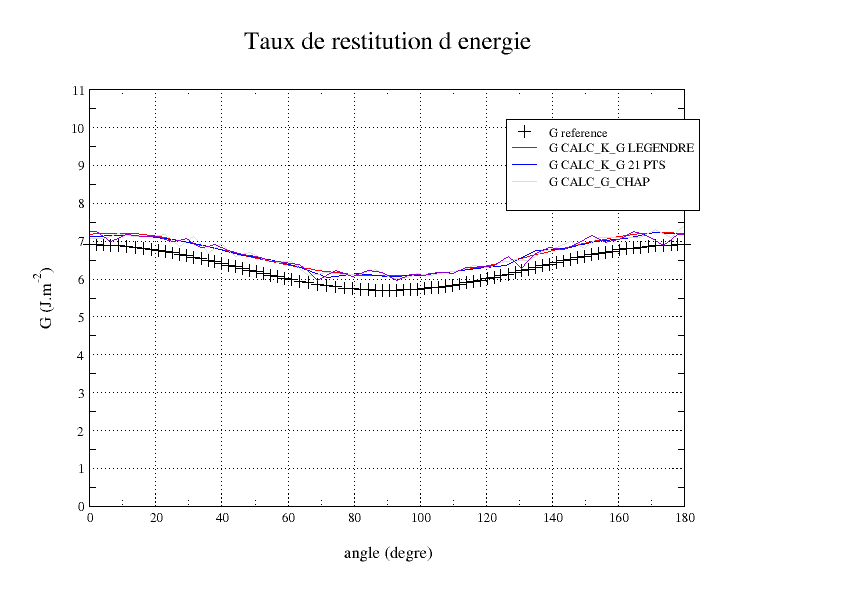
Figure 6.4-1: G along the crack bottom
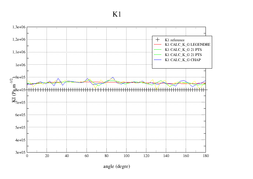
Figure 6.4-2: K1 along the crack bottom
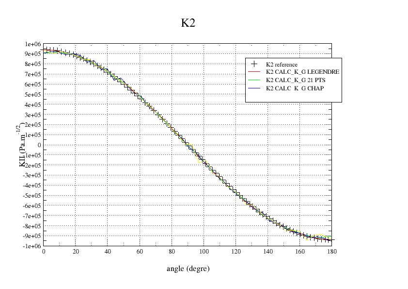
Figure 6.4-3: K2 along the crack bottom
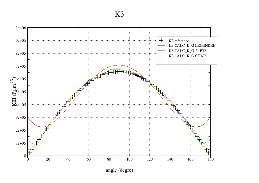
Figure 6.4-4: K3 along the crack bottom
This modeling validates the calculation of G and stress intensity factors for a 3D crack in mixed mode with the use of option NB_POINT_FOND, which makes it possible to reduce the number of points at the bottom of the crack for smoothing LINEAIRE. The use of this option is strongly recommended for smoothing LINEAIRE with a free mesh and a large number of nodes at the bottom of the crack; thus, the calculation time is significantly reduced as well as the oscillations present for smoothing LINEAIRE is used without NB_POINT_FOND. Likewise, smoothing « hat » also makes it possible to eliminate the oscillations of the values of G and K, as shown in Figure, which are all the more important for a free mesh.
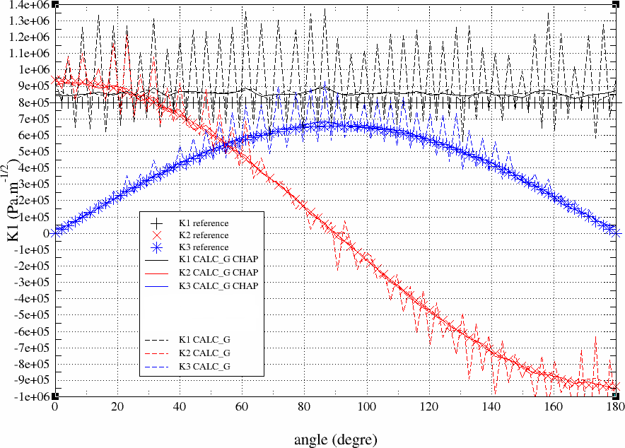
Figure 6.4-5: Comparison of the values of K1, K2, and K3 for smoothing LINEAIRE with the « hat » functions