3. Modeling A#
3.1. Characteristics of modeling#
In this modeling, the crack is meshed (case FEM). The mesh includes a torus surrounding the crack bottom.
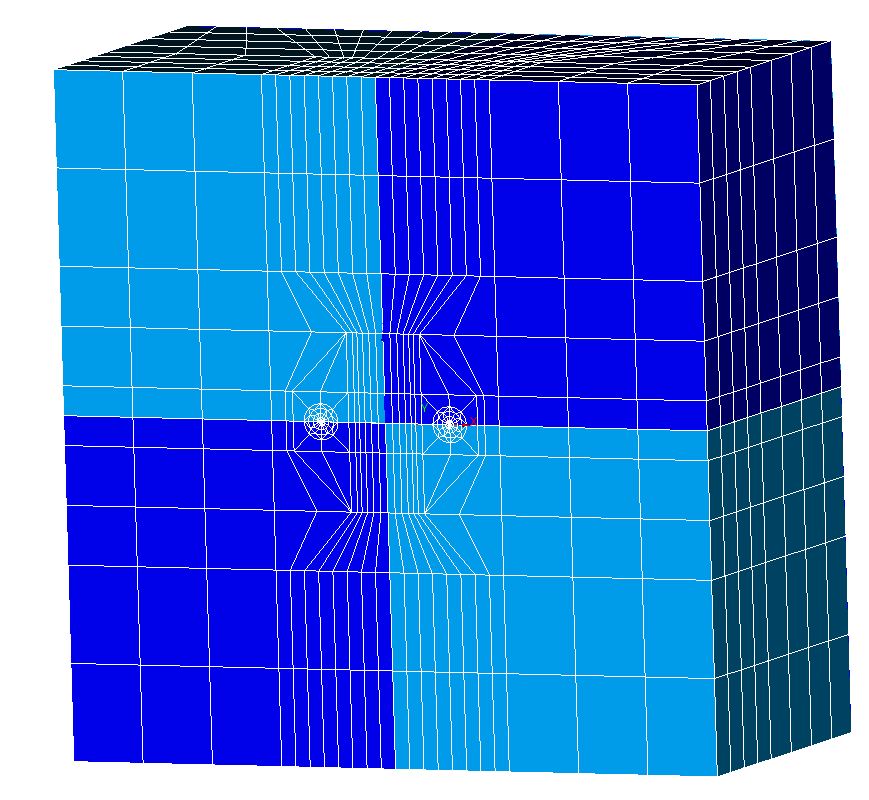
Figure 3.1-2: Structure mesh
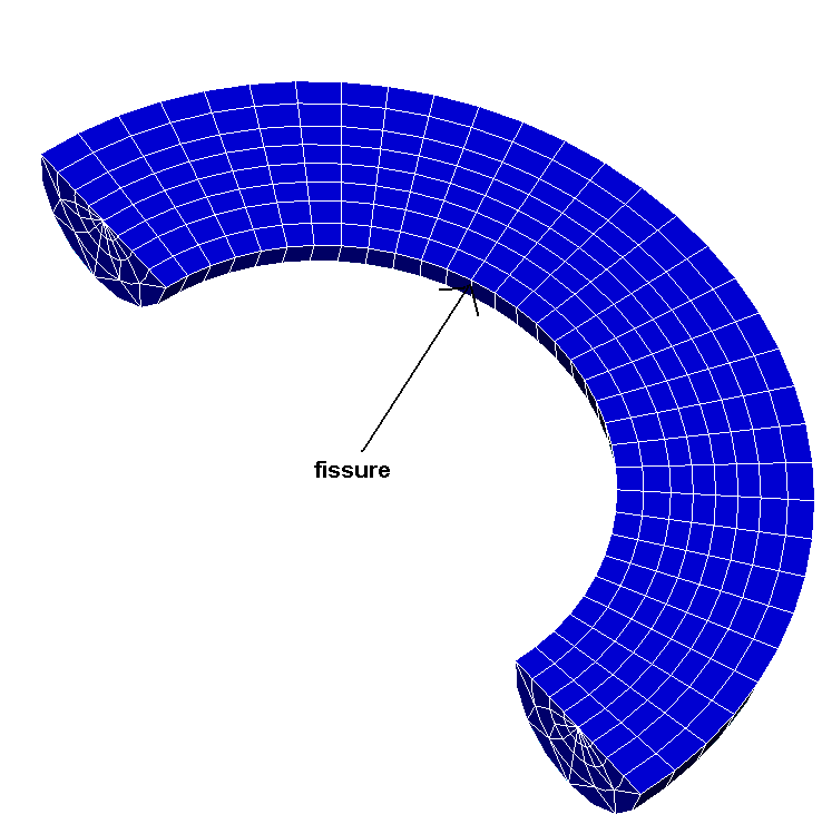
Figure 3.1-1: radiant mesh
3.2. Characteristics of the mesh#
Number of knots: 9967
Number of meshes and type: 864 PENTA15 and 1568 HEXA20
The characteristic length of an element near the crack bottom is \(\mathrm{0,12}m\).
The middle nodes of the edges of the elements touching the bottom of the crack are moved to a quarter of these edges.
3.3. Tested sizes and results#
The theta field integration crowns for command CALC_G are:
\(\text{RINF}\mathrm{=}\mathrm{0,1}m\) and \(\text{RSUP}\mathrm{=}\mathrm{0,5}m\).
We test the smoothing type LEGENDRE and the smoothing type LINEAIRE. For the latter, the results are smoothed out by a treatment that uses a hat function at the nodes, vertices of the segments at the bottom of the crack. This treatment is activated automatically in the quadratic case, to avoid oscillations in the values of G (s) in this case (see reference (2)). We then denote G « hat » (\(\widehat{G}\)) this smoothed component. The same treatment is also applied to the values of the stress intensity factors obtained by the K option of CALC_G.
The parameter ABS_CURV_MAXI of the POST_K1_K2_K3 operator is chosen so as to retain 5 nodes on the extrapolation segment.
To test the value of \({K}_{I}\) for all points at the bottom of the crack, we test the \(\mathit{min}\) and the \(\mathit{max}\) values along the bottom.
\({K}_{\mathit{II}}\) is tested only to the point where \(\omega \mathrm{=}0°\) (where \({K}_{\mathit{II}}\) is normally maximum).
\({K}_{\mathit{III}}\) is tested only to the point where \(\omega \mathrm{=}90°\) (where \({K}_{\mathit{III}}\) is normally maximum).
Theoretically, you should test the absolute value of \({K}_{\mathit{II}}\) and \({K}_{\mathit{III}}\) because the sign is arbitrary.
3.3.1. Values from CALC_G#
The values are in \(\mathit{Pa}\mathrm{.}\sqrt{m}\).
Identification |
Reference Type |
Reference Value |
% Tolerance |
|
\(\mathit{max}({K}_{I})\) |
“ANALYTIQUE” |
7,978 105 |
|
|
\(\mathit{min}({K}_{I})\) |
“ANALYTIQUE” |
7,978 105 |
4, 0% |
|
\({K}_{\mathit{II}}\) in \(\mathrm{\omega }=0°\) |
“ANALYTIQUE” |
9,386 105 |
9, 0% |
|
\({K}_{\mathit{III}}\) in \(\mathrm{\omega }=90°\) |
“ANALYTIQUE” |
6,570 105 |
3, 0% |
|
\(\widehat{G}\) in \(\omega \mathrm{=}0°\) |
“ANALYTIQUE” |
6, 906 |
|
|
\(\widehat{G}\) in \(\mathrm{\omega }=90°\) |
“ANALYTIQUE” |
5,703 |
1, 0% |
|
\(\widehat{{K}_{I}}\) in \(\omega \mathrm{=}0°\) |
“ANALYTIQUE” |
7,978 105 |
|
|
\(\widehat{{K}_{I}}\) in \(\mathrm{\omega }=90°\) |
“ANALYTIQUE” |
7,978 105 |
5, 5% |
3.3.2. Values from POST_K1_K2_K3#
The values are in \(\mathit{Pa}\mathrm{.}\sqrt{m}\).
Identification |
Reference Type |
Reference Value |
% Tolerance |
\(\mathit{max}({K}_{I})\) |
“ANALYTIQUE” |
7,978 105 |
|
\(\mathit{min}({K}_{I})\) |
“ANALYTIQUE” |
7,978 105 |
|
\({K}_{\mathit{II}}\) in \(\mathrm{\omega }=0°\) |
“ANALYTIQUE” |
9,386 105 |
|
\({K}_{\mathit{III}}\) in \(\mathrm{\omega }=90°\) |
“ANALYTIQUE” |
6,570 105 |
|
3.4. notes#
The,, and show the evolution of \(G\), \({K}_{I}\),, \({K}_{\mathit{II}}\), and \({K}_{\mathit{III}}\) along the crack background. It can be seen that the K3 is not correct. This is due to local base incorrections at the ends, which are propagated all over the front because of the polynomials in LEGENDRE.
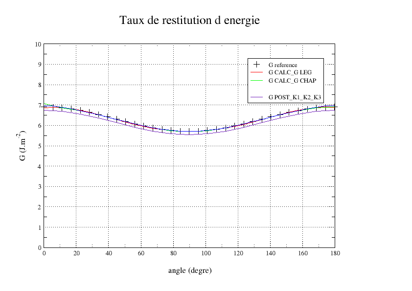
Figure 3.4-1: G along the crack bottom
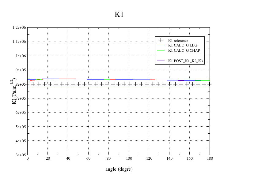
Figure 3.4-2: K1 along the crack bottom
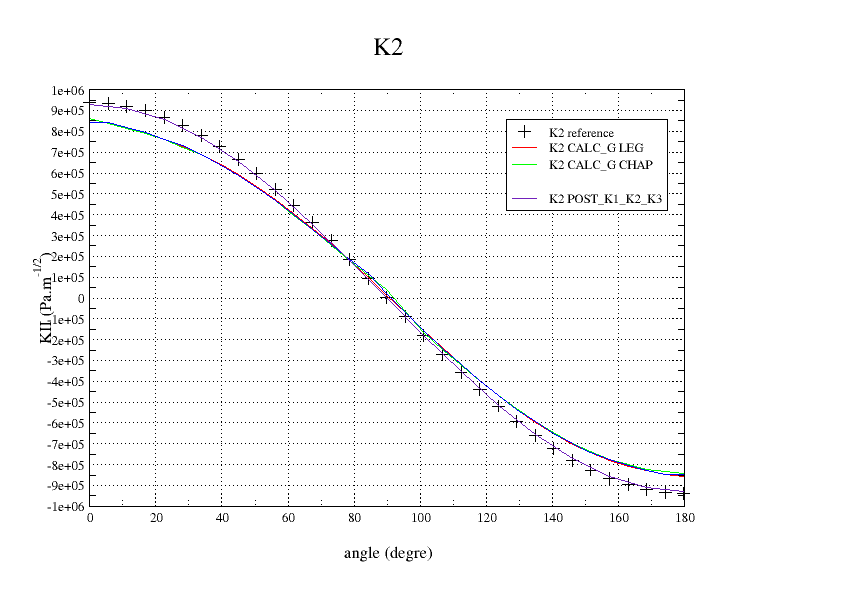
Figure 3.4-3: K2 along the crack bottom
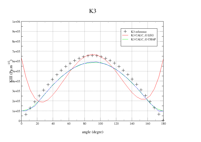
Figure 3.4-4: K3 along the crack bottom
For information, here is a comparison of SIFs along the crack bottom with a smoothing of LINEAIRE raw and with the smoothing « hat ». We can see that the raw smoothing values of LINEAIRE oscillate along the bottom. This is due to the shape functions of the quadratic elements which are different between the middle nodes and the vertex nodes and which make the interpretation of G (s) (and therefore Ki (s)) non-physical, as would be a nodal reaction on a quadratic element. The smoothing « hat » is a method for overcoming this difficulty as proposed in reference (2).
We also see that there is a bigger error on the dots at the ends of the bottom for \({K}_{\mathit{II}}\) and \({K}_{\mathit{III}}\) from CALC_G. This is due to a particular treatment of the points at the ends, which only works well if the solution is constant along the bottom. That explains why the values of \({K}_{I}\) are better. This particular treatment is only carried out for the results (\(G\), \({K}_{I}\) \({K}_{\mathit{II}}\) and \({K}_{\mathit{III}}\)) from option CALC_G OPTION K, smoothing LINEAIRE.
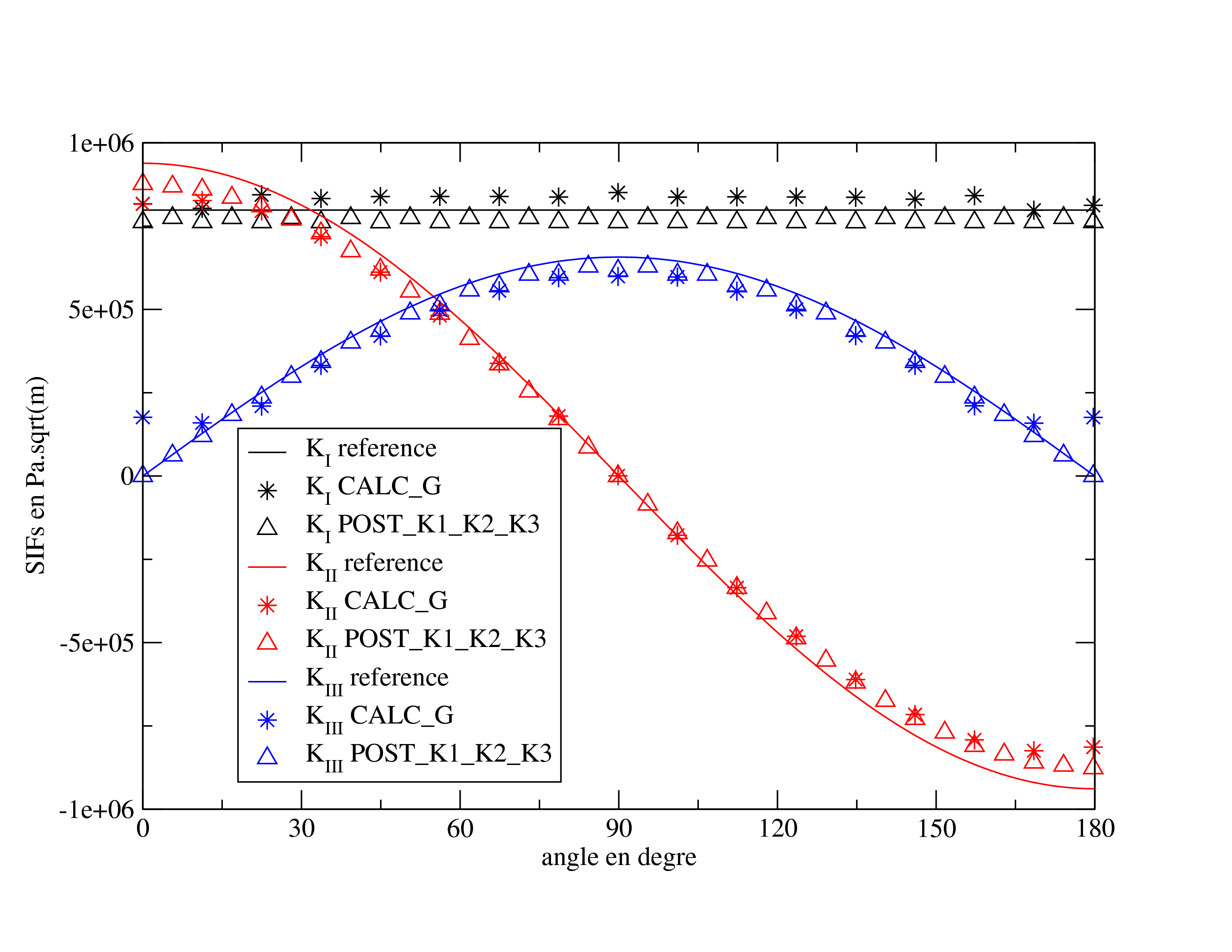
Figure 3.4-5: SIFs along the crack bottom (FEM)
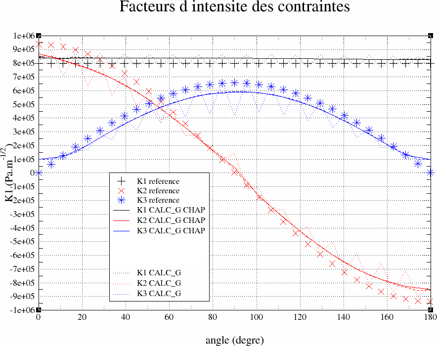
Figure 3.4-5: Comparison of the values of K1, K2, and K3 for smoothing LINEAIRE with the « hat » functions