12. Parameters for specific behaviors#

12.1. Keyword factor LEMAITRE_IRRA#

Characteristics (specific to irradiation) of the creep of fuel rods or assemblies (behavior LEMAITRE_IRRA). Elastic characteristics should be defined under the keyword ELAS or ELAS_FO.

The uniaxial form of the law of magnification is:

\({\varepsilon }_{g}(t)\mathrm{=}f(T,{\Phi }_{t})\)

where \(f\) is a function of the temperature \(T\) expressed in \(°C\) and of the fluence \({\Phi }_{t}\) expressed in \({10}^{24}\mathit{neutrons}/{m}^{2}\).

For 2D and 3D models, the law of magnification is written (Cf. [R5.03.08]):

\({\varepsilon }_{g}(t)\mathrm{=}f(T,{\Phi }_{t}){\varepsilon }_{g}^{0}\)

with: \({\epsilon }_{g}^{0}={\left(\begin{array}{ccc}1& 0& 0\\ 0& 0& 0\\ 0& 0& 0\end{array}\right)}_{{R}_{1}}\)

We must then define, using the ANGL_REP operand of the keyword MASSIF of the operator AFFE_CARA_ELEM, the local axes corresponding to the coordinate system \({R}_{1}\) (see [U4.42.01]). This operand requires 3 nautical angles of which only the first 2 are used (the third can therefore be any).

Magnification parameters are provided behind the GRAN_FO keyword.

The four keywords QSR_K, BETA, PHI_ZERO, L are filled in (the other creep parameters are identical to those of behavior LEMAITRE) and the creep behavior is then as follows:

\(\begin{array}{ccc}\dot{p}={\left[\frac{{\sigma }_{\mathrm{eq}}}{{p}^{1/m}}\right]}^{n}{(\frac{1}{K}\frac{\Phi }{{\Phi }_{0}}+L)}^{\beta }{e}^{\frac{-Q}{R(T+{T}_{0})}}& \text{}& ({T}_{O}=\mathrm{273,15}°)\end{array}\)

where \(\mathrm{\Phi }\) is the neutron flux calculated from fluence (see [R5.03.08]). \(T\) is in \(°C\).

In the case where you want the behavior not to depend on fluency, but still include the term in \(\mathrm{exp}(-Q/\mathrm{RT})\), it is possible to use the LEMAITRE_IRRA keyword in STAT_NON_LINE by entering the keyword LEMAITRE_IRRA in DEFI_MATERIAU. It is then imperative to assign UN_SUR_K, A, B, S to zero and PHI_ZERO to one. Under these conditions, it is not necessary to define a fluence field.

12.2. Keyword factor DIS_GRICRA#

This keyword makes it possible to define the parameters associated with the non-linear behavior of the connection between the grid and the rod in a fuel assembly modeled by a discrete element (cf. [R5.03.17]). The behavior that can be used in the STAT_NON_LINE and DYNA_NON_LINE commands using these parameters is DIS_GRICRA.

The input parameters for this law are as follows:

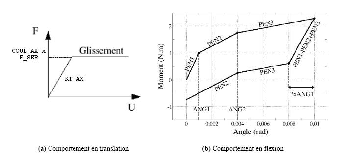
Axial sliding behavior: 6 parameters (including 2 optional parameters, purely numerical)
1. normal stiffness of the discrete KN_AX;
2. tangential stiffness (in the direction of sliding) KT_AX;
3. Coulomb friction coefficient COUL_AX;
4. clamping force F_SER (sliding limit = COUL_AX x F_SER);
5. Work hardening parameter ET_AX, the law of behavior can be equated to perfect plasticity. The work-hardening parameter is only used to ensure the convergence of the calculation and is optional, with a default value of \({10}^{-7}\);
6. stiffness parameter KP, which is paralleled by the behavior to avoid “zero pivots” in some cases. This parameter is optional with a default value of \(0\);
Rotational behavior: 8 parameters (including one purely numerical parameter)
1. successive slopes PEN1, PEN2, PEN3et PEN4 of curve \(Moment = f(angle)\);
2. angles ANG1, ANG2, and ANG3 of the inflection points of the curve;
3. work-hardening parameter ET_ROT (parameter only used to ensure the convergence of the calculation; a default value of \({10}^{-7}\) is assigned to it).
Elastic behavior in parallel: 1 parameter
1. elastic stiffness KP simulating a spring system put in parallel with the 4 discrete crosses (by default value \(0.0\))
Clamping forces may vary depending on temperature and irradiation. These dependencies are affected on slopes PEN1, PEN2, and PEN3 for rotational behavior and on the clamping force F_SER for axial sliding behavior. Dependency functions are defined directly as a FORMULE in the command file.
behavior based on a discrete element with 2 nodes (modeling DIS_TR) with degrees of freedom in translation and rotation
contact with Coulomb friction for the degrees of translation, modelled by an elastoplastic model
law of nonlinear behavior in rotation based on geometric and physical considerations (cf. [R5.03.17])

The names of the parameters followed by the suffix _FO allow you to enter the value in the form of a function.

A number of additional parameters, which are available for this behavior but which are not included in this document, are explained in [V6.04.131].

_images/10000000000002C00000013D7C38966E02944D08.png

12.3. Keyword factor DIS_CONTACT#

This keyword makes it possible to define the parameters associated with behaviors DIS_CHOC and DIS_CONTACT, non-linear shock with Coulomb friction associated with discrete elements (cf. [R5.03.17]) for models DIS_T, DIS_TR, 2D_DIS_T, 2D_DIS_TR based on meshes POI1 or SEG2 ( discrete element with 1 or 2 knots).

12.3.1. Operands#

RIGI_NOR = Kn: Value of normal shock stiffness. If RIGI_NOR is present, this value is taken into account. If it is not present, the discrete elements to which this material is assigned must have their stiffness defined elsewhere (for example using the AFFE_CARA_ELEM command with the keywords DISCRET, 2D_DISCRET or RIGI_PARASOL).
RIGI_TAN = Kt: Value of the tangential shock stiffness.
AMOR_NOR = Cn: Value of normal shock absorption.
AMOR_TAN = That: Value of tangential shock absorption.
COULOMB = mu: Value of the coefficient of friction.
DIST_1 = dist1: Characteristic distance of material surrounding the first shock node.
DIST_2 = dist2: Characteristic distance of material surrounding the second shock node (shock between two mobile structures).
JEU = d0: Distance between the shock node and an unmodelled obstacle (case of an impact between a mobile structure and an undeformable and immobile obstacle).
INST_COMP_INIT = (t0, t1): When using behavior DIS_CONTACT, cf. [R5.03.17], and when the discrete is initially compressed and in contact, it may be necessary to simulate this gradual compression in order to start from a balanced state. This keyword is used to define a ramp, if INST is the moment of calculation: \(\min\left( \max\left(0.0, (INST-t_0)∕(t_1-t_0)\right),1.0 \right)\). The value obtained multiplies the distance between the nodes or that between the node and the obstacle. The distance therefore varies between 0 to \({t}_{0}\) and its final value to \({t}_{1}\). During this phase the friction is not activated. At the end of this phase, if the discrete is compressed, the Coulomb threshold is \(\mu .N\) where \(\mathit{Fx}\) is the compression force in the discrete.
CONTACT = [“1D”|”COIN_2D”]: Allows you to define the coordinate system in which the contact is processed. By default CONTACT is managed in 1D (according to the local discrete axis). Option COIN_2D allows you to change the method of calculating the interpenetration of the 2 solids. In this case this interpenetration is calculated in the global coordinate system, and it is no longer a norm. Cf. [R5.03.17]

12.4. Keyword factor DIS_CHOC_ENDO#

This keyword makes it possible to define the parameters associated with nonlinear shock behaviors CHOC_ENDO and CHOC_ENDO_PENA associated with discrete elements (cf. [R5.03.17]) for DIS_T models based on SEG2 meshes (discrete element with 2 nodes).

12.4.1. Operands#

FX = fx

Threshold function dependent on the relative displacement of the discrete nodes.

RIGI_NOR = rn

Function describing the variation in stiffness depending on the relative displacement of the discrete nodes. This function is necessarily decreasing.

AMOR_NOR = year

Function describing the damping dependent on the relative displacement of the discrete nodes.

In all cases amortization is taken into account in the effort (cf. [R5.03.17]).

CRIT_AMOR= [“INCLUDED”|”EXCLUDED”]

Structural depreciation can be taken into account in 2 different ways. Or it is taken into account in calculating the threshold, then the effort in the discrete (if the damping is different from 0) is always less than the threshold. We therefore have a reduction in the threshold as a function of the speed of the shock. Or it is excluded from the calculation of the threshold, then the effort in the discrete can be equal to the threshold.

In all cases amortization is taken into account in the effort (cf. [R5.03.17]).

DIST_1 = dist1

Characteristic distance of material surrounding the first shock node (shock between two mobile structures).

DIST_2 = dist2

Characteristic distance of material surrounding the second shock node (shock between two mobile structures).

12.5. Keyword factor DIS_CHOC_ELAS#

This keyword makes it possible to define the parameters associated with CHOC_ELAS_TRAC nonlinear shock behaviors associated with discrete elements (cf. [R5.03.17]) for DIS_T models based on meshes SEG2 (discrete element with 2 nodes).

12.5.1. Operands#

FX = fx: Nonlinear function dependent on the relative displacement of the discrete nodes.
DIST_1 = dist1: Characteristic distance of material surrounding the first shock node (shock between two mobile structures).
DIST_2 = dist2: Characteristic distance of material surrounding the second shock node (shock between two mobile structures).

12.6. Keyword factor DIS_ECRO_CINE#

These elastoplastic material behavior parameters with non-linear kinematic work hardening, cf. [R5.03.17], are to be used with the discrete elements 2D_DIS_TR, 2D_DIS_T, DIS_TR, DIS_T (cf. operator AFFE_MODELE [U4.41.01]). The law is constructed component by component of the torsor of the resulting forces on the discrete element: there is no coupling between the force components (forces and torques), on which different characteristics can be defined; only the diagonal characteristics are affected by the behavior. The elastic stiffness \({K}_{e}\) (which is also used by the non-linear algorithm for prediction) of this law of behavior is given via the keywords K_T_D_L, K_TR_D_L, K_T_D_N, K_TR_D_N of the AFFE_CARA_ELEM [U4.42.01] command:

The quantities are all expressed in the local coordinate system of the element; it is mandatory to specify the keyword REPERE =” LOCAL “in AFFE_CARA_ELEM [U4.42.01]. The orientation of the discrete can be done in AFFE_CARA_ELEM with the usual rules using the ORIENTATION keyword.

The use of the law of behavior is done in STAT_NON_LINE or DYNA_NON_LINE under the keyword COMPORTEMENT [U4.51.11] with relationship = “DISC_ECRO_CINE”.

It is pointed out that this law of behavior is not compatible with alternating cyclic loading.

12.6.1. Operands#

LIMY_DX = fy_dx,: \({F}_{y}^{x}\): elastic limit in the force direction \(x\)
KCIN_DX = kx_dx,: \({k}_{x}\): kinematic work-hardening « stiffness » in the force direction \(x\)
PUIS_DX = n_DX,: \({n}_{x}\): power, defining the shape of the monotonic curve in the direction of effort
LIMU_DX = fu_DX,: \({F}_{u}^{x}\): kinematic work hardening limit, defining the plateau of the monotonic curve in the force direction \(x\)

12.7. Keyword factor DIS_VISC#

This non-linear viscoelastic behavior is to be used with discrete elements (cf. [R5.03.17]) 2D_DIS_TR, 2D_DIS_T, DIS_TR, DIS_T (cf. operator AFFE_MODELE [U4.41.01]). This behavior only affects the element’s local \(\mathit{dx}\) degree of freedom. The value of the elastic stiffness \({K}_{e}\) (which is also used by the non-linear algorithm for prediction) is given via the keywords K_T_D_L, K_TR_D_L, K_T_D_N, K_TR_D_Nde the command AFFE_CARA_ELEM [U4.42.01].

This viscous law of behavior can be used with the operators STAT_NON_LINE and DYNA_NON_LINE, under the keyword COMPORTEMENT [U4.51.11] with RELATION = “DIS_VISC”.

The quantities are all expressed in the local coordinate system of the element; it is mandatory to specify REPERE =” LOCAL “in AFFE_CARA_ELEM [U4.42.01]. The orientation of the discrete can be done in AFFE_CARA_ELEM with the usual rules using the orientation keyword.

12.7.1. Operands#

Behavior DIS_VISC is a non-linear viscoelastic rheological behavior, of the extended Zener type, making it possible to schematize the behavior of a uniaxial damper, applicable to the axial degree of freedom of discrete elements at two nodes (mesh SEG2) or and of discrete elements at one node (mesh POI1).

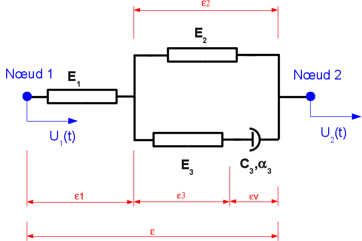
For the local direction \(x\) (and only that one) of the discrete element, 5 coefficients are provided. Their units should be in accordance with the unit of effort, the unit of lengths, and the unit of time of the problem.

K1: elastic stiffness of element 1 of the rheological model,
K2: elastic stiffness of element 2 of the rheological model,
K3: elastic stiffness of element 3 of the rheological model,
UNSUR_K1: elastic flexibility of element 1 of the rheological model,
UNSUR_K2: elastic flexibility of element 2 of the rheological model,
UNSUR_K3: elastic flexibility of element 3 of the rheological model,
PUIS_ALPHA: power of the viscous behavior of the element \(\alpha\),
\(C\): coefficient of the viscous behavior of the element.

The conditions to be met for these coefficients are (in particular to ensure the positivity and the finiteness of the tangent matrix):

\({K}_{1}⩾{10}^{-8}\); \(1/{K}_{1}⩾0\); \({K}_{3}⩾{10}^{-8}\); \(1/{K}_{3}⩾0\)

\(1/{K}_{2}⩾{10}^{-8}\); \({K}_{2}⩾0\); \(C\ge {10}^{-8}\); \({10}^{-8}\le \alpha \le 1\)

In addition, we cannot have at the same time: \(1/{E}_{1}=0\), \(1/{E}_{3}=0\) and \({E}_{2}=0\), i.e. the case of the shock absorber alone.

12.8. Keyword factor DIS_ECRO_TRAC#

Behavior DIS_ECRO_TRAC is a non-linear behavior, making it possible to schematize the behavior of a uniaxial device, along the local axis \(x\) or in the tangential plane \(\mathit{yz}\) of discrete elements at two nodes (mesh SEG2) or and of discrete elements at one node (mesh POI1).

The non-linear behavior is given by a \(F=\mathit{fonction}(\mathrm{\Delta }U)\) curve:

for a SEG2, \(\mathrm{\Delta }U\) represents the relative displacement of the 2 nodes in the local coordinate system of the element.
for a POI1, \(\mathrm{\Delta }U\) represents the absolute movement of the node in the element’s local coordinate system.
for a SEG2 or a POI1, \(F\) represents the effort expressed in the local coordinate system of the element.

This law of behavior can be used with the operators STAT_NON_LINE and DYNA_NON_LINE, under the keyword COMPORTEMENT [U4.51.11] with RELATION =” DIS_ECRO_TRAC “.

The quantities are all expressed in the local coordinate system of the element. The orientation of the discrete can be done in AFFE_CARA_ELEM with the usual rules using the orientation keyword.

12.8.1. FX operand#

The only data needed is the function describing the non-linear behavior. This function must meet the following criteria:

It is a function in the sense of code_aster: defined with the operator DEFI_FONCTION,
The interpolations on the x-axis and the y-axis are linear,
The name of the abscissa when defining the function is DX,
Extensions to the left and right of the function are excluded,
The function must be defined by**at least** 3 points,
The first point is \((\mathrm{0.0,}0.0)\) and must be given,
The function must be strictly increasing.
The derivative of the function must be less than or equal to its derivative at point \((\mathrm{0.0,0}.0)\).

Examples of defining the function:

lesX = (0.0, 0.2, 0.3, 0.50)
LesY = (0.0, 500.0, 800.0, 900.0)

fctsy1 = DEFI_FONCTION (NOM_PARA ='DX',
    ABSCISSE = the XS,
    ORDONNEE = LeSY,
)

fctsy2 = DEFI_FONCTION (NOM_PARA ='DX',
    VALE = (0.00, 0.0,
            0.20, 500.0,
            0.30, 800.0,
            0.50, 900.0),
)

The first two points of the function are used to define the elastic slope to the behavior. The x-axis and ordinate units should be consistent with those of the problem:

The unit of the abscissa must be homogeneous when displacing,
The unity of the function must be consistent with the efforts.

12.8.2. Operand FTAN#

The only data needed is the function describing the non-linear behavior. This function must meet the following criteria:

It is a function in the sense of code_aster: defined with the operator DEFI_FONCTION,
The interpolations on the x-axis and the y-axis are linear,
The name of the abscissa when defining the function is DTAN,
Extensions to the left and right of the function are excluded,
The function must be defined by**exactly ** 3 points,
The first point is \((\mathrm{0.0,}0.0)\) and must be given,
The function must be strictly increasing.
The derivative of the function must be less than or equal to its derivative at point \((\mathrm{0.0,0}.0)\).

Examples of defining the function:

LeSx = (0.0, 0.2, 0.3)
LesY = (0.0, 500.0, 800.0)

fctsy1 = DEFI_FONCTION (NOM_PARA = 'DTAN',
    ABSCISSE = the XS,
    ORDONNEE = LeSY,
)

fctsy2 = DEFI_FONCTION (NOM_PARA = 'DX',
    VALE = (0.00, 0.0,
            0.20, 500.0,
            0.30, 800.0),
)

The first two points of the function are used to define the elastic slope to the behavior. The x-axis and ordinate units should be consistent with those of the problem:

The unit of the abscissa must be homogeneous when displacing,
The unity of the function must be consistent with the efforts.

12.9. Keyword factor DIS_BILI_ELAS#

This keyword factor makes it possible to assign bilinear elastic behavior to discretes in the 3 directions of translation.

This behavior is to be used with discrete elements (cf. [R5.03.17]), 2D_DIS_T, DIS_T (cf. operator AFFE_MODELE [U4.41.01]). The law is built component by component, so there is no coupling between the force components, on which different characteristics can be defined; only the diagonal characteristics are affected by the behavior. The value of the elastic stiffness \({K}_{e}\) (which is only used by the non-linear algorithm for prediction) of this law of behavior is given via the keywords K_T_D_L, K_T_D_N of the AFFE_CARA_ELEM [U4.42.01] command.

This law of behavior can be used with the operators STAT_NON_LINE and DYNA_NON_LINE, under the keyword COMPORTEMENT [U4.51.11] with RELATION =” DISC_BILI_ELAS “.

The quantities are all expressed in the local coordinate system of the element. The orientation of the discrete can be done in the AFFE_CARA_ELEM command with the usual rules using the orientation keyword.

12.9.1. Operands#

The law of behavior is elastic bilinear and requires 3 characteristics. The units of the characteristics must be in agreement with those of the problem analyzed: \(\mathrm{k1}\) and \(\mathrm{k2}\) are homogeneous to a force per displacement, \(\mathrm{Fp}\) is homogeneous to a force.

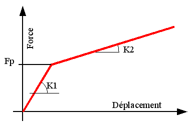
KDEB_DX = k1_dx, KDEB_DY = k1_dy, KDEB_DZ = k1_dz: The stiffness of the behavior when the effort in the discrete is less \(\mathrm{Fp}\).
KFIN_DX = k2_dx, KFIN_DY = k2_dy, KFIN_DZ = k2_dz: The stiffness of the behavior when the effort in the discrete is greater than \(\mathrm{Fp}\).
FPRE_DX = FP_DX, FPRE_DY = FP_DY, FPRE_DZ = FP_DZ: The effort that defines the transition between the 2 linear behaviors.

12.10. Keyword factor ASSE_CORN#

Description of the material characteristics associated with the behavior of a bolted joint [R5.03.32].

12.10.1. Operands#

In the following figure, plane \(\pi\) represents the assembly plane. The axis of the bolts is perpendicular to this plane. The reader will refer to [U4.42.01] AFFE_CARA_ELEM for the orientation of the coordinate system \({R}_{L}\) defining the assembly plane.

_images/1000000000000418000001B03F1BE60711349447.png

The behavior relationship of the assembly is:

nonlinear in translation following \(x\) and in rotation around \(y\).
linear according to the other degrees of freedom: \(\mathrm{DY},\mathrm{DZ},\mathrm{DRX},\mathrm{DRZ}\)

Behaviors in traction along the \(x\) axis and in rotation around the \(y\) axis.

_images/100000000000063F0000019762ECCB017D788A48.png

The behavior of the link is considered linear in the other directions:

KY: Stiffness in translation next \(Y\)
KZ: Stiffness in translation next \(Z\)
KRX: Stiffness when rotating around \(X\)
KRZ: Stiffness when rotating around \(Z\)
R_P0: Slope at origin or discharge

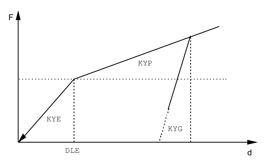
12.11. Keyword factor ARME#

Description of the material characteristics associated with the behavior of an airline armament.

The arm of each broken phase arm, represented by a discrete element, has a nonlinear force-displacement behavior consisting of the difference between the maximum displacement dlp of the end of the arm in the plastic phase and the elastic displacement limit \(dle\).

12.11.1. Operands#

KYE = key: Elastic slope up to a limited effort.
DLE = dle: Limiting displacement of elastic deformation.
KYP = kyp: Plastic slope up to limit displacement DLP.
DLP = dlp: Limiting displacement of plastic deformation 0.
KYG = kyg: Discharge slope.

12.12. Keyword factor RELAX_ACIER#

The relaxation phenomenon of steels used for prestress is regulated. The main regulations are: BPEL83, NF-EN-1992-1-1 October 2005, AFCEN - ETCC -2010,

We want to be able to model deformations that will vary slowly over time, in particular to take account of concrete creep and temperature variations. We also want to take into account the influence of temperature on relaxation phenomena.

Regularly, it would be possible to take into account the effect of concrete creep and thermal deformation by making a linear combination of the various phenomena (see regulations for more details). This approach is incompatible with a finite element calculation.

For the law of relaxation to be usable in a finite element code for structural calculations with load variations such as: concrete creep, cable tension recovery, taking into account the influence of thermal,… it must be incremental and thermodynamically correct.

The formulation adopted is based on that proposed by J.Lemaitre:

\(\mathrm{\sigma }=E.{\mathrm{\epsilon}}^{e}\) \(\mathrm{\epsilon}={\mathrm{\epsilon}}^{e}+{\mathrm{\epsilon}}^{\mathit{an}}\)

\({\dot{\varepsilon}}^{\mathrm{an}}=\langle \frac{\sigma –R({\varepsilon}^{\mathrm{an}})}{{f}_{\mathrm{prg}}\mathrm{.}k} \rangle^{n}\) with \(R \left( {\epsilon}^{an} \right)= \large {\frac{{f}_{prg}.c.{\epsilon}^{an}}{ {\left(1+{\left(b.{\epsilon}^{an} \right)}^{nr}\right)}^{\frac{1}{nr}}}}\)

The law of behavior is 1D, and only available for bar-type models, which are used to model prestress cables in operator DEFI_CABLE_BP.

To take into account the influence of temperature on relaxation, all the coefficients of the law can be functions of temperature.

Note:: The parameters \(c\), \(b\), \(n\) and \(\mathit{nr}\) are unitless, and therefore independent of the units used during the study. \(k\) is dimensionless compared to \({f}_{\mathit{prg}}\) so in relation to the constraints, but not in relation to time. Indeed \({\dot{\mathrm{\epsilon}}}^{\mathit{an}}\) is homogeneous to \({[s]}^{-1}\), if the time unit is in seconds. So if we know \(k\) for a speed in a unit of time, it is necessary to convert its value in relation to the unit of time used during the study.

12.12.1. Operands#

\(\bf f_{prg}\): Cable breaking stress. This quantity is optional, as it can also be defined in materials BPEL_ACIER or ETCC_ACIER and in this case \({f}_{\mathit{prg}}\) is a constant. The value/function given under RELAX_ACIER_CABL takes precedence.
ECOU_K, ECOU_N: Corresponding respectively to the coefficients k, n, in the equation.
ECRO_N, ECRO_B, ECRO_C: Corresponding respectively to the coefficients n, b, c, in the equation.

12.13. Keyword factor CABLE_GAINE_FROT#

This material is for CABLE_GAINE items only. It makes it possible to define the friction behavior between a cable and its sheath or between a cable and the surrounding concrete. It is possible to consider a slippery, rubbing or adherent cable. For its use, see behavior KIT_CG in U4.51.11.

12.13.1. Operands#

TYPE: This operand allows you to define whether it is a slippery, rubbing or adherent cable.
PENA_LAGR = pen,: This operand defines the penalty coefficient to be taken into account. (See R3.08.10, §6.1 for more details).
FROT_LINE = fl: Rectilinear coefficient of friction.
FROT_COURB = fc: Curved friction coefficient.

12.14. Keyword factor FONDA_SUPERFI#

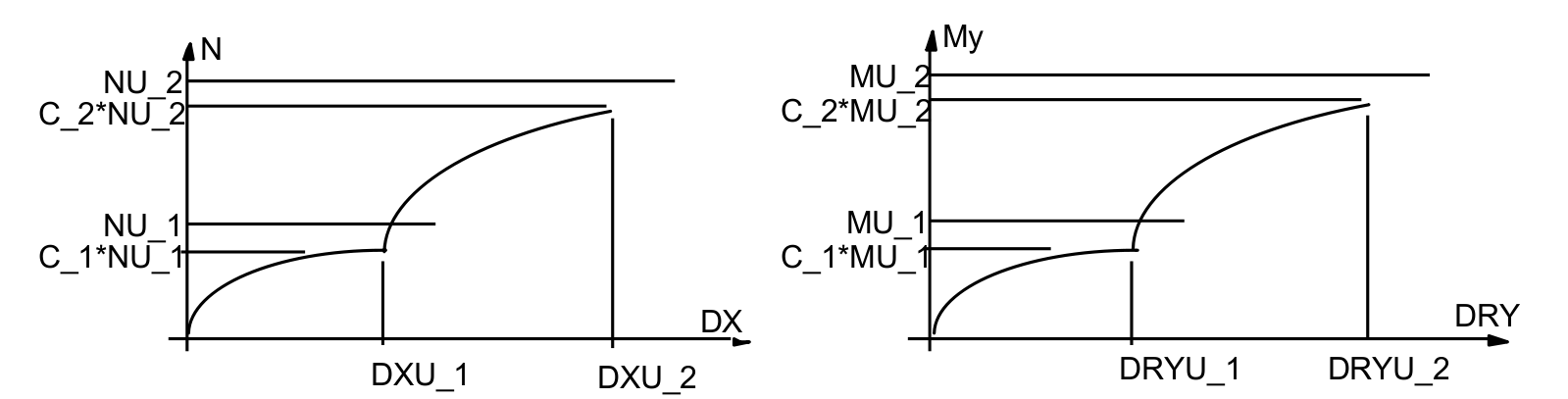
The nonlinear elastoplastic behavior of a rectangular surface foundation subjected to three-dimensional static or seismic stress uses the parameters defined for this material, cf. [R5.03.17] and [R5.03.31]. This law of behavior applies to 3D discrete elements composed of a single translational and rotating node (DIS_TR) assigned a diagonal stiffness matrix (K_TR_D_N) using the relationship FONDATION called by the nonlinear problem solving operators STAT_NON_LINE [R5.03.01] or DYNA_NON_LINE [R5.05.05].

12.14.1. Operands#

LONG_X: Length lx along the local x axis of the foundation (mandatory).
LONG_Y: Length ly along the local y axis of the foundation (mandatory).
PHI = phi: Angle of friction in degrees at the soil/foundation interface (mandatory).
COHESION = check: Cohesion at the soil/foundation interface (homogeneous with translational stiffness, optional). By default equal to 0.
RAID_GLIS: RG sliding work hardening stiffness (optional). By default equal to 0.
GAMMA_REFE: Parameter gr for kinematic work hardening (homogeneous at the opposite of a distance, optional). By default equal to 0.
CP_SERVICE: Elastic limit force cps of the foundation (mandatory).
CP_ULTIME: Ultimate CPU limit strength of the foundation (optional). By default equal to 0.
DEPL_REFE: Reference compaction dr for isotropic work hardening of the load-bearing capacity criterion (optional). By default equal to 0.
RAID_CP_ [X|Y|RX|RY] = rcp [x|y|rx|ry]: Stiffness of kinematic work hardening in translation or in rotation according to x or y of the load-bearing capacity criterion (homogeneous to a stiffness in translation, optional). By default equal to 0.
GAMMA_CP_ [X|Y|RX|RY] = gcp [x|y|rx|ry]: Parameter of kinematic work hardening in translation or in rotation according to x or y of the load-bearing capacity criterion (homogeneous at the opposite of a distance, optional). By default equal to 0.
DECOLLEMENT: Parameter for activating the detachment mechanism if equal to “OUI”. (Optional and by default “NON”).

12.15. Keyword factor JONC_ENDO_PLAS#

These parameters are used to define, based on the analysis of the reinforced concrete section: geometry and characteristics of materials, cf. [R5.03.17], the non-linear behavior of an off-plane flexural connection, a junction between a wall and a floor or a raft, in reinforced concrete, cf. [U2.02.03], to be applied to discrete elements of type DIS_TR on cells SEG2, at two nodes. Moments \(M\), like stiffness, are therefore expressed in units of torque (length * force).

12.15.1. Operands#

KE: Elastic rotational stiffness \({K}_{e}>0\). We will take the same value as that entered in AFFE_CARA_ELEM (DISCRET =( _F (_F (CARA =” K_TR_D_ *”, REPERE =” LOCAL “,…),),),).
KP: Plastic work hardening slope \({K}_{p}\le {K}_{e}\).
KDP: Tangent stiffness \({K}_{d}^{\text{+}}\in \left[{K}_{e},{K}_{p}\right]\) in the damaging phase for positive bending.
KDM: Tangent stiffness \({K}_{d}^{\text{-}}\in \left[{K}_{e},{K}_{p}\right]\) in the damaging phase for negative bending.
RDP: Rotation damage threshold \({\theta }_{d}^{\text{+}}>0\) in positive bending.
RDM: Rotation damage threshold \({\theta }_{d}^{\text{-}}<0\) in negative bending.
MYP: Plasticity threshold \({M}_{y}^{\text{+}}⩾{K}_{e}{\theta }_{d}^{\text{+}}\) in positive flexure.
MYM: Plasticity threshold \({M}_{y}^{\text{-}}⩽{K}_{e}{\theta }_{d}^{\text{-}}\) in negative flexure.