4. General elastic characteristics#
4.2. Keyword ELAS_VISCO#
The keyword ELAS_VISCO makes it possible to define isotropic viscoelastic materials for a given frequency. It is simply the definition of an elastic material whose elasticity modules are complex.
4.2.1. G/NU operands#
G = g
Complex shear module.
NU = naked
Complex Poisson’s ratio.
4.2.2. Operand RHO#
RHO = rho
Density. No verification of the order of magnitude.
4.3. Keyword factor ELAS_FLUI#
The keyword ELAS_FLUI makes it possible to define the equivalent density of a tubular structure with internal and external fluid, taking into account the confinement effect.
This operation is part of the study of the dynamic behavior of a configuration such as a « bundle of tubes under transverse flow ». The study of the behavior of the beam is reduced to the study of a single tube representative of the entire beam. Cf. [U4.35.02].
The equivalent density of structure \({\rho }_{\mathit{eq}}\) is defined by:
\(\begin{array}{cc}{\rho }_{\mathrm{eq}}=\frac{1}{({d}_{e}^{2}-{d}_{i}^{2})}\left[{\rho }_{\mathrm{i.}}{d}_{i}^{2}+{\rho }_{\mathrm{t.}}({d}_{e}^{2}-{d}_{i}^{2})+{\rho }_{e}\mathrm{.}{d}_{e}^{2}\right]& \\ {d}_{\mathrm{eq}}^{2}=\frac{2\mathrm{.}{C}_{m}\mathrm{.}{d}_{e}^{2}}{\pi }& \end{array}\)
\({\rho }_{i}\), \({\rho }_{e}\), \({\rho }_{t}\) are respectively the density of the fluid, of the external fluid and of the structure.
\({d}_{e}\), \({d}_{i}\) are the outer and inner diameter of the tube respectively.
\({C}_{m}\) is an added mass coefficient (which defines confinement).
4.3.1. Operands RHO /E/NU#
RHO = rho
Density of the material.
E = yg
Young’s module.
NU = naked
Poisson’s ratio.
4.3.2. Operands PROF_RHO_F_INT/PROF_RHO_F_EXIT/COEF_MASS_AJOU#
PROF_RHO_F_INT = rhoi
A concept of type [function] defining the density profile of the internal fluid along the tube. This function is parameterized by the curvilinear abscissa.
PROF_RHO_F_EXT = rhoe
Type concept [function] defining the density profile of the external fluid along the tube. This function is parameterized by the curvilinear abscissa, “ABSC”.
COEF_MASS_AJOU = fund_cm
[Function] type concept produced by operator FONC_FLUI_STRU [U4.35.02].
This constant function, parameterized by the curvilinear abscissa, provides the value of the added mass coefficient \({C}_{m}\).
4.4. Keyword factor CABLE#
Definition of the nonlinear, constant elastic characteristic for cables: two different elastic behaviors in tension and in compression, defined by the Young E and EC modules (compression modulus).
The standard characteristics of elastic material are to be entered under the keyword factor ELAS.
4.4.1. Elasticity operands#
◊ EC_SUR_E = ECSE
Relation of modules to compression and traction. If the compression modulus is zero, the global linear system at the movements can become singular. This is the case when a node is only connected to cables and the cables all come into compression.
4.5. Tags factor ELAS_ORTH, ELAS_ORTH_FO, ELAS_VISCO_ORTH#
Definition of orthotropic elastic characteristics that are constants or functions of temperature for isoparametric massive elements or the constituent layers of a composite [R4.01.02]. It is possible to define constant orthotropic viscoelastic characteristics (ELAS_VISCO_ORTH) at a given frequency, the modules to be filled in are then complex.
4.5.1. Elasticity operands#
To define the orthotropy coordinate system \((\text{L},\text{T},\text{N})\) linked to the elements, the reader will refer to:
for massive isoparametric elements in the documentation [U4.42.01] AFFE_CARA_ELEM MASSIF keyword,
for composite shell elements to the documentation [U4.42.01] AFFE_CARA_ELEM keyword COQUE as well as to the documentation [U4.42.03] DEFI_COMPOSITE keyword ORIENTATION.
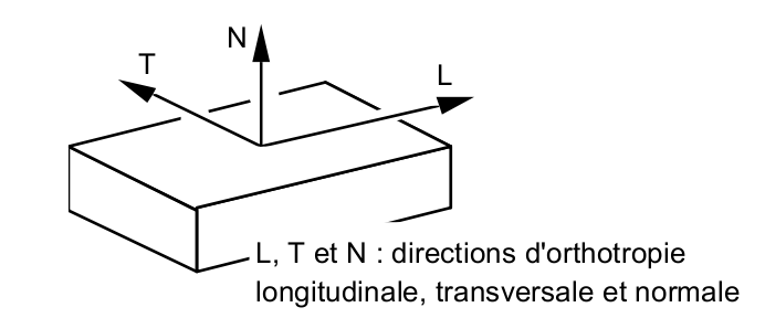
E_L = ygl Longitudinal Young's Modulus
E_T = ygtTransverse Young's module.
E_N = ygnNormal Young's module.
GL_T = glt Shear modulus in the :math:`\text{LT}` plane.
G_TN = gtn Shear module in the :math:`\text{TN}` plane.
G_LN = gln Shear modulus in the :math:`\text{LN}` plane.
Note:
For shells, transverse shear modules are not mandatory; in this case, we calculate in a thin shell by assigning infinite stiffness to the transverse shear (elements DST, , DSQet Q4G) .
NU_LT = zero Poisson's ratio in the :math:`\text{LT}` plane.
Important notes:
\(\mathit{nult}\) does not equal to \(\mathit{nutl}\). In fact, we have the relationship: \(\mathit{nutl}=\frac{\mathit{ygt}}{\mathit{ygl}}\mathrm{.}\mathit{nult}\)
\(\mathit{nult}\) should be interpreted as follows:
if we exert traction along the axis \(L\) giving rise to a deformation along this axis equal to \({\epsilon }_{L}=\frac{{\sigma }_{L}}{\mathit{ygl}}\) , we have a deformation along the axis \(T\) equal to: \({\epsilon }_{T}=-\mathit{nult}\mathrm{.}\frac{{\sigma }_{L}}{\mathit{ygl}}\) .
The various elasticity coefficients E_L, * G_LNet NU_LNne cannot be chosen in any way: physically, a non-zero deformation must always cause a strictly positive deformation energy. This results in the fact that the Hooke matrix must be positive definite. The operator DEFI_MATERIAU calculates the eigenvalues of this matrix and sounds an alarm if this property is not verified.
For 2D models, as the user has not yet chosen his MODELISATION (D_PLAN, C_PLAN,…), we check the positivity of the matrix in the various cases.
NU_TN = nutn Poisson's Ratio in plan :math:`\text{TN}`.
NU_LN = no Poisson's ratio in the :math:`\text{LN}` plane.
The remark made for NU_LT should be applied to these last two coefficients. This is how we have the relationships:
\(\begin{array}{}\mathrm{nunt}=\frac{\mathrm{ygn}}{\mathrm{ygt}}\mathrm{.}\mathrm{nutn}\\ \mathrm{nunl}=\frac{\mathrm{ygn}}{\mathrm{ygt}}\mathrm{.}\mathrm{nuln}\end{array}\)
Note:
In the command file it is necessary to enter complex numbers even if the imaginary part is zero, for example if nult is real, it requires” complex (nult,0) “
4.5.2. Special case of cubic elasticity#
Cubic elasticity corresponds to an elasticity matrix of the form:
\(\begin{array}{cccccc}{y}_{1111}& {y}_{1122}& {y}_{1122}& & & \\ {y}_{1122}& {y}_{1111}& {y}_{1122}& & & \\ {y}_{1122}& {y}_{1122}& {y}_{1111}& & & \\ & & & {y}_{1212}& & \\ & & & & {y}_{1212}& \\ & & & & & {y}_{1212}\end{array}\)
Given the cubic symmetry, it remains to determine 3 coefficients:
\({E}_{L}={E}_{N}={E}_{T}=E,{G}_{\text{LT}}={G}_{\text{LN}}={G}_{\text{TN}}=G,{\nu }_{\text{LN}}={\nu }_{\text{LT}}={\nu }_{\text{LN}}=\nu\)
To reproduce cubic elasticity with ELAS_ORTH, simply calculate the orthotropy coefficients such that the elasticity matrix obtained is of the form above:
\(\begin{array}{}{y}_{1111}=\frac{E(1-{\nu }^{2})}{(1-3{\nu }^{2}-2{\nu }^{3})}\\ {y}_{1122}=\frac{E\nu (1+\nu )}{(1-3{\nu }^{2}-2{\nu }^{3})}\\ {y}_{1212}={G}_{\text{LT}}={G}_{\mathrm{ln}}={G}_{\mathrm{TN}}\end{array}\)
so as long as \((1-3{\nu }^{2}-2{\nu }^{3})\ne 0\) (i.e. \(\nu\) different from \(0.5\)).
\(\frac{{y}_{1122}}{{y}_{1111}}=\frac{\nu }{1-\nu }\) which provides \(\begin{array}{ccc}\text{}& \text{}& \text{}\\ \nu & \text{=}& \frac{1}{1+\frac{{y}_{1111}}{{y}_{1122}}}\end{array}\) then \(E={y}_{1111}\frac{(1-3{\nu }^{2}-2{\nu }^{3})}{(1-{\nu }^{2})}\)
4.5.3. Operand RHO#
RHO = rho
Density.
4.5.4. Operands ALPHA_L/ALPHA_T/ALPHA_N#
ALPHA_L = he
Longitudinal mean thermal expansion coefficient.
ALPHA_T = said
Mean transverse coefficient of thermal expansion.
ALPHA_N = din
Normal mean thermal expansion coefficient.
4.5.5. Operands TEMP_DEF_ALPHA/PRECISION#
Refer to paragraph [§3.1.4]. This keyword becomes mandatory as soon as ALPHA_L, or ALPHA_T or ALPHA_N has been entered.
4.5.6. Breakup criteria#
XT = trl
Criterion of failure in traction in the longitudinal direction (first direction of orthotropy).
XC = collar
Criterion of rupture under compression in the longitudinal direction.
YT = trt
Criterion of failure in traction in the transverse direction (second direction of orthotropy).
YC = cost
Criterion of rupture under compression in the transverse direction.
S_LT = cis
Criterion for shear failure in plane \(\text{LT}\).
4.5.7. Operands AMOR_ALPHA/AMOR_BETA/AMOR_HYST#
See Operands AMOR_ALPHA/AMOR_BETA/AMOR_HYST.
- note
In the case of multi-layer shells (use of DEFI_COMPOSITE), these parameters are not taken into account.
4.6. Tags factor ELAS_ISTR, ELAS_ISTR_FO, ELAS_VISCO_ISTR#
Definition of constant elastic characteristics (ELAS_ISTR) or temperature functions in the case of transverse isotropy for isoparametric massive elements (ELAS_ISTR_FO). It is possible to define constant transverse isotropic viscoelastic characteristics (ELAS_VISCO_ISTR) at a given frequency, the modules to be filled in are then complex.
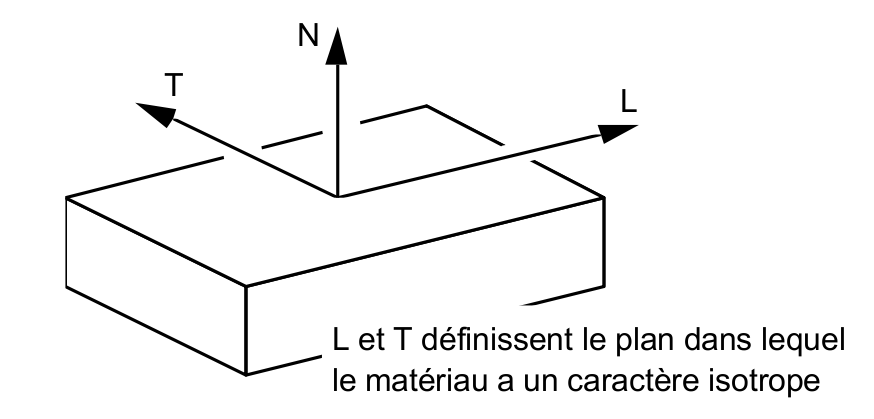
Using the same notations as for orthotropy, transverse isotropy here means that the isotropy is in plane \((\text{L},\text{T})\) and that the orthotropy is therefore carried by the direction \(\text{N}\) [R4.01.02]. The reader’s attention may be drawn to the fact that this convention differs from a usual convention which designates by « longitudinal direction » the direction of orthotropy of isotropic transverse materials.
4.6.1. Elasticity operands#
To define a \((\text{L},\text{T},\text{N})\) coordinate system linked to the elements and defining the transverse isotropy of the material, the latter being isotropic in the \(\text{LT}\) plane, the reader will refer to the documentation [U4.42.01] AFFE_CARA_ELEM keyword MASSIF.
Note:
The directions \(\text{L}\) and \(\text{T}\) are arbitrary in the plan \(\text{LT}\) .
E_L = ygl
Young’s module in plane \(\text{LT}\).
E_N = ygn
Normal Young’s modulus.
GL_N = gln
Shear modulus in plane \(\text{LN}\).
Note:
The shear modulus in the plane \(\text{LT}\) is defined by the usual formula for isotropic materials: \(G=\frac{E}{2(1+\nu )}\) or here \(\mathrm{glt}=\frac{\mathrm{ygl}}{2(1+\mathrm{nult})}\) .
NU_LT = null
Poisson’s ratio in plane \(\text{LT}\).
NU_LN = null
Poisson’s ratio in plane \(\text{LN}\).
Important notes:
\(\mathrm{nult}=\mathrm{nutl}\) since the material has an isotropic character in plane \(\text{LT}\) , but \(\mathrm{nuln}\) does not equal to \(\mathrm{nunl}\) .
We have the relationship: \(\mathrm{nunl}=\frac{\mathrm{ygn}}{\mathrm{ygl}}\mathrm{.}\mathrm{nuln}\)
\(\mathrm{nunl}\) should be interpreted as follows:
if we exert traction along the axis \(N\) giving rise to a tensile deformation along this axis equal to \({\varepsilon }_{N}=\frac{{\sigma }_{N}}{\mathrm{ygn}}\) , we have a compression along the axis \(L\) equal to: \(\mathrm{nunl}\mathrm{.}\frac{{\sigma }_{N}}{\mathrm{ygn}}\) .
The various elasticity coefficients E_L, * G_LNet * ** NU_LN cannot be chosen in any way: physically, a non-zero deformation must always cause a strictly positive deformation energy. This results in the fact that the Hooke matrix must be positive definite. The operator DEFI_MATERIAU calculates the eigenvalues of this matrix and sounds an alarm if this property is not verified.
For 2D models, as the user has not yet chosen his MODELISATION (D_PLAN, C_PLAN,…), we check the positivity of the matrix in the various cases.
4.6.2. Operand RHO#
RHO = rho
Density.
4.6.3. Operands ALPHA_L/ALPHA_N#
ALPHA_L = he
Average thermal expansion coefficient in plane \(\text{LT}\).
ALPHA_N = din
Normal mean thermal expansion coefficient.
4.6.4. Operands TEMP_DEF_ALPHA/PRECISION#
Refer to paragraph [§3.1.4]. This keyword becomes mandatory as soon as the ALPHA_L or ALPHA_N keyword is entered.
4.8. Keyword factor ELAS_MEMBRANE#
ELAS_MEMBRANE allows the user to directly provide the coefficients of the elasticity matrix of anisotropic membranes in linear elasticity.
The elastic stiffness matrix relating membrane stresses to membrane deformations for membrane elements is defined as follows:
\({\mathrm{H}}_{\mathrm{M}}=\left(\begin{array}{ccc}H1111& H1122& H1112\\ H1122& H2222& H2212\\ H1112& H2212& H1212\end{array}\right)\)
In the case of an isotropic elastic membrane, the matrix must be found:
\(\frac{\mathit{Eh}}{1-{\nu }^{2}}\left(\begin{array}{ccc}1& \nu & 0\\ \nu & 1& 0\\ 0& 0& \left(\frac{1-\nu }{2}\right)\end{array}\right)\)
These coefficients are to be provided in the local coordinate system of the element, defined under the keyword factor MEMBRANE of the AFFE_CARA_ELEM [U4.42.01] command. These coefficients have the dimension of one force per meter. Recall that the following notation conventions are used for membrane deformations and stresses, and that the coefficients of the previous matrix must be adapted accordingly:
\(\epsilon =\left(\begin{array}{c}{\epsilon }_{11}\\ {\epsilon }_{22}\\ \sqrt{2}{\epsilon }_{12}\end{array}\right)\) \(\sigma =\left(\begin{array}{c}{\sigma }_{11}\\ {\sigma }_{22}\\ \sqrt{2}{\sigma }_{12}\end{array}\right)\)
The user can also specify an isotropic thermal expansion coefficient alpha and a mass per unit area.
4.9. Keyword factor ELAS_HYPER#
Definition of hyper-elastic characteristics of the Signorini type [R5.03.19]. The Piola Kirchhoff \(\mathrm{S}\) stresses are related to the Green-Lagrange deformations by:
\(\mathrm{S}=\frac{\partial \mathrm{\Psi }}{\partial \mathrm{E}}\) with: \(\mathrm{\Psi }={C}_{10}\left({I}_{1}-3\right)+{C}_{01}\left({I}_{2}-3\right)+{C}_{20}{\left({I}_{1}-3\right)}^{2}+\frac{1}{2}K{\left(J-1\right)}^{2}\) and \({I}_{1}={I}_{c}{J}^{-\frac{2}{3}}\text{, }{I}_{2}={\mathit{II}}_{c}{J}^{-\frac{4}{3}}\text{, }J={\mathit{III}}_{c}^{\frac{1}{2}}\)
where \({I}_{c}\), \({\mathit{II}}_{c}\), and \({\mathit{III}}_{c}\) are the 3 right Cauchy-Green tensor invariants.
4.9.1. C01, C10, and C20 operands#
C01 = c01, C10 = c10, C20 = c20
The three coefficients of the polynomial expression for hyperelastic potential. Unity is \(N/{m}^{2}\).
If \({\mathrm{C}}_{01}\) and \({\mathrm{C}}_{20}\) are zero, we get a Neo-Hookian material.
If only \({\mathrm{C}}_{20}\) is zero, a Mooney-Rivlin material is obtained.
The material is elastic and cannot be compressed into small deformations if we take \({\mathrm{C}}_{10}\) and \({\mathrm{C}}_{01}\) such as \(6\left({\mathrm{C}}_{01}+{\mathrm{C}}_{10}\right)=E\), where \(E\) is Young’s modulus.
4.9.2. NU and K operand#
NU= naked
Poisson’s ratio. We check that \(\mathrm{-}1<\mathit{nu}<0.5\).
K = k
Compressibility module.
These two parameters are mutually exclusive (when one of the two parameters is entered, the other cannot be entered). They quantify the almost compressibility of the material. We use the compressibility module \(K\) provided by the user, if it exists. Otherwise we calculate \(K\) by:
\(K=\frac{6\left({C}_{01}+{C}_{10}\right)}{3\left(1-2\nu \right)}\).
We can take \(\mathit{nu}\) close to \(0.5\) but never strictly equal (to the nearest machine precision). If \(\mathit{nu}\) is too close to \(0.5\), an error message prompts the user to check their Poisson’s ratio or compressibility module. The greater the compressibility module, the more incompressible the material is.
4.9.3. Operand RHO#
RHO = rho
Real constant density (we do not accept a function-type concept). No verification of the order of magnitude.
4.10. Keyword factor ELAS_HYPER_VISC#
Definition of visco-hyper-elastic characteristics [R5.03.19]. Viscous flow is taken into account by adding a Prony series of order \(n\) to the second Piola Kirchoff tensor PK2 in the long run. The Piola Kirchhoff \(\mathrm{S}\) stresses are related to the Green-Lagrange deformations by:
\(\mathrm{S}=\frac{\partial \mathrm{\Psi }}{\partial \mathrm{E}}+\sum_{i=1}^NH_{i}\) with: \(\mathrm{\Psi }={C}_{10}\left({I}_{1}-3\right)+{C}_{01}\left({I}_{2}-3\right)+{C}_{20}{\left({I}_{1}-3\right)}^{2}+\frac{1}{2}K{\left(J-1\right)}^{2}\)
and:math: `H_ {i} |_ {t} |_ {t+triangle t} =exp (-frac {dt} {tau_ {i}}) H_ {i} |_ {t} +g_itau_ {i} (1-tau_ {i}} (1-exp (-frac {dt} {i}}))frac {(S^ {iso}}))frac {(S^ {iso} |) _ {t+triangle t} -S^ {iso} |_ {t})} {dt} `.
4.10.1. C01, C10, and C20 operands#
C01 = c01, C10 = c10, C20 = c20
The three coefficients of the polynomial expression of the long-term hyperelastic potential. Unity is \(N/{m}^{2}\).
If \({\mathrm{C}}_{01}\) and \({\mathrm{C}}_{20}\) are zero, we get a Neo-Hookian material.
If only \({\mathrm{C}}_{20}\) is zero, a Mooney-Rivlin material is obtained.
The material is elastic and cannot be compressed into small deformations if we take \({\mathrm{C}}_{10}\) and \({\mathrm{C}}_{01}\) such as \(6\left({\mathrm{C}}_{01}+{\mathrm{C}}_{10}\right)=E\), where \(E\) is Young’s modulus.
4.10.2. K operand#
K = k
Compressibility module. It quantifies the almost compressibility of the material. The bigger \(K\), the more incompressible the material is. The user can calculate it from the Poisson’s ratio and the hyperelastic potential coefficients of the instantaneous behavior as in the case of ELAS_HYPER, cf.§ 4.9.2.
4.10.3. G operand and TAU#
G = g
Length list \(n\) (order of development of the Prony series) of long-term shear relaxation modules.
TAU = tau
Length list \(n\) containing relaxation times.
4.11. Keyword factor SECOND_ELAS#
Definition of the isotropic linear elastic characteristics of the second gradient model proposed by Mindlin and detailed in the documentation [R5.04.03]. This behavior is used for second dilation gradient regularization models (* _ DIL).
4.11.1. A1 operand#
This parameter defines the material characteristics of the law described in document [R5.04.03].
4.12. Keyword factor ELAS_GLRC#
Definition of the constant linear elastic characteristics of a homogenized plate for laws GLRC_DM and GLRC_DAMAGE.
4.12.1. Operands E_M/ NU_M /E_F/ NU_F/BT1/BT2#
E_M = em
Young’s modulus of the membrane. We check that \({E}_{m}\ge 0\).
NU_M = num
Membrane Poisson’s ratio. We check that \(-1.\le {\nu }_{m}\le 0.5\).
E_F = ef
Young’s modulus of flexure. We check that \({E}_{f}\ge 0\).
NU_F = nine
Poisson’s ratio of flexure. We check that \(-1.\le {\nu }_{f}\le 0.5\).
BT1 = bt1 and BT2 = bt2
In the case where finite elements support the calculation of shear forces, these operands are used to define the elastic transverse shear stiffness matrix. The \(V\) shear forces are linked to the distortions \(\gamma\) by:
\(\mathrm{V}=\left(\begin{array}{cc}\mathit{BT}1& 0\\ 0& \mathit{BT}2\end{array}\right)\mathrm{.}\gamma\)
The other operands are identical to those for linear elasticity, cf. § 4.1.
4.13. Keyword factor ELAS_DHRC#
Definition of the constant linear elastic characteristics of a homogenized plate for law DHRC.
4.13.1. A0 operands#
A0= a0
Components (\(21\) supra-diagonal terms) of the symmetric elasticity tensor \({A}^{0}\) membrane-flexure of the plate before damage, of order \(4\), in the frame coordinate system \((x,y)\), in Voigt notations, identified by homogenization: first in membrane, then in flexure (unit of force per unit of length for membrane terms (unit of force per unit of length for membrane terms), unit of force for coupled membrane-flexure terms, and unit of force times unit of flexure (unit of force per unit of length for membrane terms), unit of force for coupled membrane-flexure terms, and unit of force times unit of length (for flexure terms):
\((\begin{array}{cccccc}{A}_{\mathrm{xxxx}}^{\mathrm{0mm}}& {A}_{\mathrm{xxyy}}^{\mathrm{0mm}}& {A}_{\mathrm{xxxy}}^{\mathrm{0mm}}& {A}_{\mathrm{xxxx}}^{\mathrm{0mf}}& {A}_{\mathrm{xxyy}}^{\mathrm{0mf}}& {A}_{\mathrm{xxxy}}^{\mathrm{0mf}}\\ \text{}& {A}_{\mathrm{yyyy}}^{\mathrm{0mm}}& {A}_{\mathrm{yyxy}}^{\mathrm{0mm}}& {A}_{\mathrm{yyxx}}^{\mathrm{0mf}}& {A}_{\mathrm{yyyy}}^{\mathrm{0mf}}& {A}_{\mathrm{yyxy}}^{\mathrm{0mf}}\\ \text{}& \text{}& {A}_{\mathrm{xyxy}}^{\mathrm{0mm}}& {A}_{\mathrm{xyxx}}^{\mathrm{0mf}}& {A}_{\mathrm{xyyy}}^{\mathrm{0mf}}& {A}_{\mathrm{xyxy}}^{\mathrm{0mf}}\\ \text{}& \text{}& \text{}& {A}_{\mathrm{xxxx}}^{\mathrm{0ff}}& {A}_{\mathrm{xxyy}}^{\mathrm{0ff}}& {A}_{\mathrm{xxxy}}^{\mathrm{0ff}}\\ \text{}& \text{}& \text{}& \text{}& {A}_{\mathrm{yyyy}}^{\mathrm{0ff}}& {A}_{\mathrm{yyxy}}^{\mathrm{0ff}}\\ \text{}& \text{}& \text{}& \text{}& \text{}& {A}_{\mathrm{xyxy}}^{\mathrm{0ff}}\end{array})\)
The other operands are identical to those for linear elasticity, cf. § 4.1.
4.15. Keyword factor CZM_ELAS#
This keyword factor makes it possible to specify the parameters of the elastic interface law CZM_ELAS_MIX (see [R7.02.11]).
4.15.1. Operands RIGI_TAN, RIGI_NOR, RIGI_NOR_TRAC, and RIGI_NOR_COMP#
The RIGI_TANpermet keyword is to define tangential stiffness at the interface (transverse isotropic). The RIGI_NORpermet keyword is to define normal stiffness at the interface, provided that it is the same in tension and compression. It is also possible to choose different normal stiffness in tension and in compression via the keywords RIGI_NOR_TRACet RIGI_NOR_COMP respectively.
In the absence of these keywords, the corresponding rigidities are zero.
4.15.2. Operand ADHE_NOR#
This keyword makes it possible to characterize the normal behavior at the interface. The default value, “ELAS”, corresponds to an elastic response (potentially distinct in tension and compression); the stiffness is then defined via RIGI_NORou, alternatively, RIGI_NOR_TRACet RIGI_NOR_COMP. The value “UNILATER” refers to a contact type behavior (zero interpenetration) when closed and elastic when opened (equivalent to an infinite stiffness in compression). Finally, the value “PARFAITE” states that the normal displacement jump is zero, that is, there is perfect grip in the direction normal to the interface (equivalent to infinite normal stiffness).
4.15.3. Operand ADHE_TAN#
This keyword makes it possible to characterize the behavior tangent to the interface. The default value, “ELAS”, corresponds to an elastic response; the stiffness ktest is then defined via RIGI_TAN. The value “PARFAITE” states that the tangent displacement jump (slip) is zero, that is, there is perfect adherence in the direction tangent to the interface (equivalent to infinite tangential stiffness).
4.15.4. Operand PENA_LAGR_ABSO#
This keyword (mandatory) allows you to enter the value of the increased Lagrangian coefficient of increase, cf. [R7.02.11]. Unlike other models, it is not provided in relation to other parameters (because they can all be zero) but in an absolute way. Its dimension is that of a pressure per unit of length.