6. Behaviors related to damage and breakage

6.1. Tags factor ROUSSELIER, ROUSSELIER_FO

Definition of the coefficients of the Rousselier ductile fracture behavior model (cf. [R5.03.06] and [R5.03.07]). This model can be used for small deformations, large deformations, and viscoplasticity (keyword VISC_SINH)

Briefly, for an elastoplastic increment, the following is solved:

\(\{\begin{array}{cc}\frac{{\sigma }_{\mathit{eq}}}{\rho }-R\left(p\right)+D{\sigma }_{1}f\mathrm{exp}\left(\frac{{\sigma }_{H}}{{\sigma }_{1}}\rho \right)=0& \text{éq 5.1-1}\\ \sigma =\rho \mathrm{\Lambda }\left(\epsilon -{\epsilon }^{p}\right)\hfill & \phantom{\rule{2em}{0ex}}\\ \dot{{\epsilon }_{p}}=\dot{p}\rho \frac{\partial f}{\partial \sigma }\hfill & \phantom{\rule{2em}{0ex}}\\ \dot{f}=3\left(1-f\right){\epsilon }_{H}^{p}\hfill & \phantom{\rule{2em}{0ex}}\end{array}\)

with \(\{\begin{array}{cc}\frac{\partial f}{\partial \sigma }=\frac{1}{\rho }\left(\frac{3}{2}\frac{\stackrel{~}{\sigma }}{{\sigma }_{\mathit{eq}}}+\frac{\mathit{Df}}{3}\mathrm{exp}\left(\frac{{\sigma }_{H}}{{\sigma }_{1}\rho }\right)\right)& \phantom{\rule{2em}{0ex}}\\ \rho =\frac{1-f}{1-{f}_{0}}\hfill & \text{éq 5.1-2}\end{array}\)

\(R(p)\) entered via the traction curve (keyword TRACTION).

With ROUSSELIER’s model-specific \(D,{\sigma }_{\mathrm{1,}}{f}_{0}\) material coefficients.

These various parameters may depend on the temperature, in this case the keyword ROUSSELIER_FO will be used.

It is possible to complete the model by using the following quantities:

• critical porosity \({f}_{c}\) beyond which cavity growth is accelerated:

\(\dot{f}=3A(1-f){\epsilon }_{H}^{p}\text{}\mathit{si}f>{f}_{c}\)

two additional characteristics are then required: \({f}_{c}\) and \(A\).

• the porosity limit \({f}_{l}\) beyond which the material is considered broken. The behavior is then replaced by an imposed drop in constraints:

\(\dot{\sigma }=-\lambda E\frac{\sigma }{\mid \sigma \mid }\mid \dot{\varepsilon }\mid \text{}\mathrm{si}f={f}_{l}\) (with \(E\) defined under ELAS).

two additional characteristics are then required: \({f}_{1}\) and \(\lambda\).

• the volume germination rate of cleavage cracks \({A}_{n}\), modifying equations [éq 5.1-1] and [éq 5.1-2] as follows.

\(\mathrm{\{}\begin{array}{c}\frac{{\sigma }_{\mathit{eq}}}{\rho }\mathrm{-}R(p)+D{\sigma }_{1}(f+{A}_{n}p)\mathrm{exp}(\frac{{\sigma }_{H}}{{\sigma }_{1}\rho })\mathrm{=}0\\ \rho \mathrm{=}\frac{1\mathrm{-}f\mathrm{-}{A}_{n}p}{1\mathrm{-}{f}_{0}}\end{array}\)

These last five parameters are independent of temperature.

The following correspondence table should be used:

Modeling	Keywords
\(D\)	D
\({\sigma }_{1}\)	SIGM_1
\({f}_{0}\)	PORO_INIT
\({f}_{c}\)	PORO_CRIT dp
\(A\)	PORO_ACCE
\({A}_{n}\)	YEAR
\({f}_{l}\)	PORO_LIMI
\(\lambda\)	D_SIGM_EPSI_NORM

In version SIMO_MIEHE the law of behavior requires redistribution when the plastic deformation increment is greater than the \(\mathit{dp}\) value provided behind the key word DP_MAXI.

The keyword BETA must be filled in with behaviors ROUSS_PR or ROUSS_VISC to take into account adiabatic heating: it sets the proportion of plastic energy that is effectively transformed into heat.

The user is given the choice via the keyword PORO_TYPE to change the porosity formulation according to the plastic deformation or the total deformation. It was noticed that for a low initial porosity \({f}_{0}\), the behavior at the beginning of evolution changes strongly depending on this parameter. Thus PORO_TYPE is affected by 1 (porosity in plastic deformation), 2 (porosity in total deformation).

6.1.1. Help with use

The Rousselier model has been the subject of numerous developments and has several variants named ROUSSELIER, ROUSS_PR and ROUSS_VISC (these models are available in the STAT_NON_LINE command via the RELATION keyword). Thus, each of its models requires particular knowledge from the « user » point of view. In order to clarify this, a summary table is set out below, along with various remarks.

		ROUSSELIER []	ROUSS_PR []	ROUSS_VISC []
COMPORTEMENT	SIMO_MIEHE	xxxx
	GDEF_LOG	xxxx
	PETIT_REAC		xxxx	xxxx
MODELISATION	3D	xxxx	xxxx	xxxx
	Axisymmetric	xxxx	xxxx	xxxx
	CP		xxxx	xxxx
	RFP	xxxx	xxxx	xxxx
	INCOMPRESSIBLE (xxx_inco_ugp)	xxxx

Notes:

When using incompressible elements (refer to doc [R3.06.08]), the keyword C_GONF must be entered in DEFI_MATERIAU under operand NON_LOCAL (refer to §5.6 and the ssnap122a test case).

For a formulation with three fields UPG, it is preferable to use the MUMPS solver to solve linear systems. In addition, the user should be warned that it is advisable to consider as a convergence criterion, a convergence criterion by reference constraint under the keyword RESI_REFE_RELA.

6.2. Keyword factor GTN

This keyword makes it possible to define the coefficients of the GTN model (behavioral relationships GTN and VISC_GTN) for the part related to the evolution of porosity, cf. [R5.03.29]. It covers the three aspects of ductile rupture, namely the phases of germination, growth, and cavity coalescence.

6.2.1. Operands

The cavity germination phase (nucleation in English, hence the prefix NUCL in the keywords) is modelled by a contribution to porosity, noted \({f}^{\mathit{nuc}}\), the other contribution being linked to the growth of cavities \({f}^{\mathit{growth}}\):

\(\dot{f}={\dot{f}}^{\mathit{growth}}+{\dot{f}}^{\mathit{nuc}}\text{;}{\dot{f}}^{\mathit{growth}}=\left(1-f\right)\mathrm{tr}{\dot{\mathrm{E}}}^{\mathrm{p}}\text{avec}f(0)={f}_{0}\)

The evolution of the germination porosity is a function of the work hardening variable \(\kappa\) and of the cumulative plastic deformation according to the following incremental model:

\({\dot{f}}^{\mathit{nuc}}={B}_{n}\left(\mathrm{\kappa }\right)\dot{\mathrm{\kappa }}+{b}_{0}{\dot{E}}_{\mathit{eq}}^{p}H({E}_{\mathit{eq}}^{p}-{E}_{c}^{p})\text{;}{B}_{n}(\mathrm{\kappa })=\frac{{f}_{N}}{{s}_{N}\sqrt{2\mathrm{\pi }}}\mathrm{exp}\left[-\frac{1}{2}{\left(\frac{\mathrm{\kappa }-{\mathrm{\kappa }}_{N}}{{s}_{N}}\right)}^{2}\right]+\frac{{c}_{0}}{{\mathrm{\kappa }}_{f}-{\mathrm{\kappa }}_{i}}{\mathrm{\chi }}_{[{\mathrm{\kappa }}_{i}\text{;}{\mathrm{\kappa }}_{f}]}\)

where \(H\) designates the Heaviside function (zero for a strictly negative argument, equal to 1 for a positive argument) and \({\chi }_{I}\) the characteristic function of a set \(I\) (equal to 1 in \(I\), zero elsewhere).

In the absence of declaration of the germination parameters, the function \(B\) and \({b}_{0}\) are null so that there is then no germination.

Cavity growth is described by the evolution of plasticity, governed by a threshold function that relies on an equivalent constraint \({T}_{\text{*}}\). The latter is defined implicitly by the following equation, in which \(\mathrm{T}\) designates the constrained tensor specific to kinematics GDEF_LOG:

\({\left(\frac{{T}_{\mathit{eq}}}{{T}_{\text{*}}}\right)}^{2}+2{q}_{1}{f}_{\text{*}}\mathrm{cosh}\left({q}_{2}\frac{3}{2}\frac{{T}_{H}}{{T}_{\text{*}}}\right)-1-{q}_{1}{f}_{\text{*}}=0\)

where \({T}_{\mathit{eq}}\) refers to vonMises’s equivalent constraint and \({T}_{H}\) refers to a third of the trace of \(T\).

Coalescence results (under load) in an acceleration of the evolution of effective porosity \({f}_{\text{*}}\) according to the following relationship:

\(\{\begin{array}{cc}\mathrm{si}\phantom{\rule{2em}{0ex}}f\le {f}_{c}& {f}_{\text{*}}=f\hfill \\ \mathrm{si}\phantom{\rule{2em}{0ex}}f>{f}_{c}& {f}_{\text{*}}={f}_{c}+{\mathrm{\delta }}_{c}(f-{f}_{c})\end{array}\)

Again, there will be no coalescence mechanism (\({f}_{\text{*}}=f\)) if the corresponding parameters are not filled in. The slope \({\delta }_{c}\) can be provided directly or recalculated if it is preferred to enter the porosity at break \({f}_{r}\) such as \({q}_{1}{f}_{\text{*}}({f}_{r})=1\).

Finally, two additional parameters activate techniques for regularizing the model to reinforce its robustness: ENDO_CRIT_VISC and ENDO_CRIT_RUPT. By designating the value \({q}_{1}{f}_{\text{*}}\) as « damage », the model VISC_GTNl introduces “damage viscosity threshold \({d}_{v}\) beyond which the loss of viscosity resulting from the damage is limited, which makes it possible to maintain a certain degree of viscous regularization in order to absorb stress shocks. Moreover, to avoid trying to solve the equations of the model for damage that is too close to 1 (they degenerate for \(d=1\)), it is possible to prematurely force the rupture of the point in question beyond damage \({d}_{r}\). By default, it is calculated according to the numerical precision requested by the user (RESI_INTE_RELA) but this can be too restrictive and lead to excessive division of time steps.

6.3. Tags VENDOCHAB/VENDOCHAB_FO

Definition of the coefficients of the viscoplastic model with scalar damage of Chaboche confer [R5.03.15]). It is a multiplicative straining-viscosity behavior coupled with isotropic damage. Briefly, relationships are:

\(\{\begin{array}{c}\sigma =\left(1-D\right)A{\epsilon }^{e}\text{et}{\epsilon }^{e}=\epsilon -{\epsilon }^{\mathit{th}}-{\epsilon }^{p}\\ \dot{{\epsilon }^{p}}=\frac{3}{2}\dot{p}\frac{\stackrel{~}{\sigma }}{{\sigma }_{\mathit{eq}}}\text{avec}\dot{p}=\frac{\dot{r}}{\left(1-D\right)}\hfill \\ \dot{r}={\left(\frac{{\sigma }_{\mathit{eq}}-S\left(1-D\right)}{\left(1-D\right){\mathit{Kr}}^{1/M}}\right)}^{N}\hfill \\ \dot{D}={\left(\frac{\chi \left(\sigma \right)}{A}\right)}^{R}{\left(1-D\right)}^{-k\left(\chi \left(\sigma \right)\right)}\hfill \end{array}\)

with \(D\), the isotropic damage scalar variable and:

\(\chi \left(\sigma \right)=\alpha {J}_{0}\left(\sigma \right)+\beta {J}_{1}\left(\sigma \right)+\left(1-\alpha -\beta \right){J}_{2}\left(\sigma \right)\)

where:

\({J}_{0}\left(\sigma \right)\) is the maximum principal stress

\({J}_{1}\left(\sigma \right)=\mathit{Tr}\left(\sigma \right)\)

\({J}_{2}\left(\sigma \right)={\sigma }_{\mathit{eq}}\)

\(\langle x\rangle\): positive part of \(x\), \(\stackrel{~}{\sigma }\) constraint deviator and \({\sigma }_{\mathrm{eq}}\) the Von Mises constraint.

The table below summarizes the matches between the equation symbols and the Aster keywords.

Material parameter	Symbol in equations	Keyword in Aster
Viscoplasticity threshold	\(S\)	“SY”
Coefficient 1 of equivalent creep stress	\(\alpha\)	“ALPHA_D”
Coefficient 2 of equivalent creep stress	\(\beta\)	“BETA_D”
Damage Law Coefficient	\(A\)	“A_D”
First exponent of the law of damage	\(R\)	“R_D”
Second exponent of the law of damage	\(k\left[\chi \left[\sigma \right]\right]\)	“K_D”

note

The parameter K_D can be defined as a constant, a function of a parameter “TEMP” or a sheet (temperature and stress variable \(\chi \left(\sigma \right)\)). In this case, use DEFI_NAPPE with “TEMP” as the first parameter for the temperature in \(°C\) and as the second parameter “X” (required) for the constraints in \(\mathit{MPa}\). If K_D only depends on \(\chi \left(\sigma \right)\), you must use DEFI_NAPPE anyway, for example by entering the same data set twice under stress for two different temperature values.

6.4. Tags VISC_ENDO/VISC_ENDO_FO

Definition of the coefficients of the Lemaître visco-plastic model with scalar damage VISC_ENDO_LEMA cf. [R5.03.15]), which corresponds to a simplified and optimized version of the model VENDOCHAB (cf. [U4.51.11]).

\(\{\begin{array}{c}\sigma =\left(1-D\right)A{\epsilon }^{e}\text{et}{\epsilon }^{e}=\epsilon -{\epsilon }^{\mathit{th}}-{\epsilon }^{p}\\ \dot{{\epsilon }^{p}}=\frac{3}{2}\dot{p}\frac{\stackrel{~}{\sigma }}{{\sigma }_{\mathit{eq}}}\text{avec}\dot{p}=\frac{\dot{r}}{\left(1-D\right)}\hfill \\ \dot{r}={\left(\frac{\frac{{\sigma }_{\mathit{eq}}}{(1-D)}-{\sigma }_{y}}{{\mathit{Kr}}^{1/M}}\right)}^{N}\text{}\dot{D}={\left(\frac{{\sigma }_{\mathit{eq}}}{A\left(1-D\right)}\right)}^{R}\hfill \end{array}\)

The table below summarizes the correspondence between the equation symbols and the keywords.

Material parameter	Symbol in equations	Keyword
Viscoplasticity threshold	\({\sigma }_{y}\)	“SY”
Damage Law Coefficient	\(A\)	“A_D”
First exponent of the law of damage	\(R\)	“R_D”

6.5. Tags HAYHURSTet HAYHURST_FO

Definition of the coefficients of the Hayhurst visco-plastic model, to describe the elasto-viscoplastic behavior of austenitic steels, with scalar damage in hyperbolic sine, a function of the maximum principal stress, isotropic work hardening and a viscous law in hyperbolic sine:

\(\{\begin{array}{c}\sigma =\left(1-D\right)C{\epsilon }^{e}\text{et}{\epsilon }^{e}=\epsilon -{\epsilon }^{\mathit{th}}-{\epsilon }^{p}\hfill \\ \dot{{\epsilon }^{p}}=\frac{3}{2}\dot{p}\frac{\stackrel{~}{\sigma }}{{\sigma }_{\mathit{eq}}}\text{avec}\dot{p}=\dot{{\epsilon }_{0}}\text{sinh}\left(\frac{{\sigma }_{\mathit{eq}}(1-H)}{K\left(1-D\right)(1-\varphi )}\right)\phantom{\rule{4em}{0ex}}\text{avec}\phantom{\rule{4em}{0ex}}\dot{\varphi }=\frac{{k}_{c}}{3}{(1-\varphi )}^{4}\hfill \\ \text{si S\_EQUI\_D}=0\phantom{\rule{4em}{0ex}}\dot{D}=\dot{{A}_{0}}\text{sinh}\left(\frac{\alpha \text{<}{\sigma }_{I}{\text{>}}_{\text{+}}+{\sigma }_{\mathit{eq}}(1-\alpha )}{{\sigma }_{0}}\right)\hfill \\ \text{si S\_EQUI\_D}=1\phantom{\rule{4em}{0ex}}\dot{D}=\dot{{A}_{0}}\text{sinh}\left(\frac{\alpha \text{<}\mathit{tr}(\sigma ){\text{>}}_{\text{+}}+{\sigma }_{\mathit{eq}}(1-\alpha )}{{\sigma }_{0}}\right)\hfill \\ H={H}_{1}+{H}_{2}\hfill \\ \dot{{H}_{i}}=\frac{{h}_{i}}{{\sigma }_{\mathit{eq}}}\left({H}_{i}^{\text{*}}-{\delta }_{i}{H}_{i}\right)\dot{p}\phantom{\rule{4em}{0ex}}i=\mathrm{1,2}\hfill \end{array}\)

6.6. Tag factor RUPT_FRAG, RUPT_FRAG_FO

The Frankfurt and Marigo fracture theory makes it possible to model the appearance and propagation of brittle fracture cracks. It is based on the Griffith criterion, which compares the return of elastic energy and the energy dissipated during the creation of a cracked surface, provided by the GC keyword. These are the concepts that are used to describe the break in cohesive zone models, by defining other concepts specific to certain laws. RUPT_FRAG is the keyword used to define the material parameters of cohesive behavior laws, CZM_xxx (with the exception of CZM_TRA_MIX and CZM_LAB_MIX) (see [R7.02.11]).

6.6.1. G_C operand

The energy dissipated is proportional to the crack area created, the coefficient of proportionality being the critical energy density of material \({G}_{c}\).

6.6.2. Operand SIGM_C

Critical stress at the origin from which the crack will open and the stress between the lips will decrease.

6.6.3. Operand PENA_ADHERENCE

Small parameter for regularizing the stress to zero (for more details see [R7.02.11]).

note

The parameters SIGM_C and PENA_ADHERENCE are only mandatory in the case of xxx_ JOINT models. They are not used for the Griffith criterion, which is why they appear to be optional at the catalog level.

6.6.4. Operand PENA_CONTACT

Small contact regularization parameter.

6.6.5. Operands PENA_LAGR and RIGI_GLIS

Lagrangian penalization parameter (\(\mathit{pla}\ge 1.01\)) and stiffness in sliding mode.

Operand CINEMATIQUE

Determine the opening modes authorized by the interface law for law CZM_TAC_MIX. “UNILATER” means that the two volumes on either side of the interface cannot interpenetrate, “GLIS_2D “that the two volumes can only slide in the plane tangential to the interface, and” GLIS_1D “that they can only slide in one direction.

The tangent coordinate system in question is defined using the keyword factor MASSIFde AFFE_CARA_ELEM [U4.42.01]. In the case of one-dimensional sliding, the only possible sliding direction is defined by the second vector of the rotated coordinate system (\(\mathit{Oy}\)).

6.7. Keyword factor NON_LOCAL

This keyword factor makes it possible to specify the characteristics necessary for the use of non-local behavioral models for which the response of the material is no longer defined at the level of the material point but at that of the structure, see also AFFE_MODELE [U4.41.01] and [R5.04].

6.7.1. Operands LONG_CARA/C_GRAD_VARI/COEF_RIGI_MINI/C_GONF/PENA_LAGR

LONG_CARA = long

Determine the characteristic length or length scale internal to the material. Do not use with non-local damage laws with damage gradient GRAD_VARI.

C_GRAD_VARI = long

Nonlocality parameter for the internal variable gradient formulation, present in free energy in the form \(c/2{\left(\nabla a\right)}^{2}\). It determines the characteristic length of the damage zone. For use only with non-local damage laws with damage gradient GRAD_VARI.

COEF_RIGI_MINI = key

For its part, it has an algorithmic role since it sets, for damage models that degrade the stiffness of the material, the proportion of the initial stiffness (Young’s modulus) defined under ELAS (0.1% for example) below which the damage mechanism is stopped: this residual stiffness makes it possible to preserve the well-posed nature of the elastic problem.

C_GONF = bloated

In the Rousselier model, the softening character is supported by porosity, which has a purely hydrostatic effect. To control the location, the idea is to regulate the problem only on this part and therefore to regulate the swelling variable if modeling INCO_UPG is used.

PENA_LAGR = pena

Penalization parameter used for models with gradients of internal variables (_ GRAD_VARI) and second gradient (_ DIL), which makes it possible to control the coincidence between a field at the nodes (degrees of freedom specific to the non-local) and a field at Gauss points (internal variable or deformation).

A default value of 1000 is set. For modeling _ DIL it is not recommended to reduce this value (loss of precision for resolution). For modeling GRAD_VARI this parameter corresponds to the multiplier \(r\) of the quadratic term of penalization in free energy: \(r/2{\left(\alpha -a\right)}^{2}\). It is up to the user to adjust its value according to the law used.

PENA_LAGR_INCO = pena_inco

Penalization parameter used for gradient models of internal variables in large deformations (_ GRAD_INCO), which makes it possible to strengthen the kinematic relationship between the degree of freedom of swelling and the change in volume as a result of the deformation. Numerical tests in the case of a ductile fracture problem lead to the recommendation of a value of the order of ten times the initial elastic limit. A value that is too low (or zero) can lead to the appearance of plastic localization bands. An excessively high value leads to numerical locking in incompressibility, which is precisely what this enriched kinematics seeks to limit.

6.8. Keyword factor CZM_LAB_MIX

This keyword factor makes it possible to specify the parameters of the steel-concrete interface law CZM_LAB_MIX (see [R7.02.11]).

6.8.1. Operand SIGM_C

Maximum stress bearable by the steel-concrete interface.

6.8.2. Operand GLIS_C

Sliding for which the stress at the interface is maximum.

6.8.3. Operands ALPHA and BETA

Shape parameters of the steel-concrete adhesion law. alpha typically varies between 0 and 1, while beta is positive.

6.8.4. Operands PENA_LAGR

Lagrangian penalization parameter (\(\mathit{pla}\ge 1.01\)).

6.8.5. Operand CINEMATIQUE

Determine the sliding modes allowed by the interface law. “UNILATER” means that the two volumes on either side of the interface cannot interpenetrate, “GLIS_2D “that the two volumes can only slide in the tangential plane to the interface, and” GLIS_1D “means that they can only slide in one direction.

The tangent coordinate system in question is defined using the keyword factor MASSIF from AFFE_CARA_ELEM [U4.42.01]. In the case of one-dimensional sliding, the only possible sliding direction is defined by the second vector of the rotated coordinate system (\(\mathit{Oy}\)).

6.9. Keyword factor RUPT_DUCT

These material characteristics are intended to define the behavior of a ductile cohesive crack with the law of behavior CZM_TRA_MIX see [R7.02.11].

6.9.1. G_C operand

The energy dissipated is proportional to the crack area created, the coefficient of proportionality being the critical energy density of material \({G}_{c}\).

6.9.2. Operand SIGM_C

Critical stress at the origin from which the crack will open.

6.9.3. Operands COEF_EXTR and COEF_PLAS

Form parameters of the cohesive law CZM_TRA_MIX see [R7.02.11].

6.9.4. Operands PENA_LAGR and RIGI_GLIS

Lagrangian penalization parameter (\(\mathit{pla}\mathrm{\ge }.01\)) and stiffness in sliding mode.

6.10. Keyword factor RANKINE

Simplified modeling of concrete dam joints is based on this material [R7.01.39]. This is a criterion for perfect plasticity in traction involving the components of the main stresses: \({\mathrm{\sigma }}_{i=\mathrm{1,2,3}}\le {\mathrm{\sigma }}_{t}\). When a main constraint reaches threshold value \({\mathrm{\sigma }}_{t}\), the joint opens in that direction. It should be noted that the plastic deformation thus created is not reversible, the model therefore does not make it possible to represent the reclosing of the joint and is only valid on a monotonous loading path.

6.10.1. Operand SIGMA_T

Traction threshold (positive value).

6.11. Keyword factor JOINT_MECA_RUPT

The modeling of dam joints is based on these material characteristics, cf. [R7.01.25]. The hydrostatic pressure due to the possible presence of fluid in the joint is taken into account. Two industrial procedures are also implemented: claving - injecting concrete under pressure between the supports of the structure and sawing - dam sawing in order to release compression stresses. This material keyword is used by the law of behavior of the same name: JOINT_MECA_RUPT.

6.11.1. K_N operand

Normal tensile stiffness.

6.11.2. K_T operand

Tangential stiffness.

6.11.3. Operand SIGM_MAX

Maximum critical stress at which the crack opens and the stress between the lips decreases. This stress is often referred to as tensile strength.

6.11.4. Operand ALPHA

Parameter for regulating tangential damage. The critical opening length at which the tangential stiffness falls to zero is defined as follows:

\({L}_{\mathit{CT}}={L}_{C}\mathrm{tan}(\mathit{ALPHA}\mathrm{\pi }/4)\)

Operand PENA_RUPTURE

Fragile break smoothing parameter. The maximum opening before complete breakage is given by \({L}_{C}=\mathrm{SIGM}\text{\_}\mathrm{MAX}(1+\mathrm{PENA}\text{\_}\mathrm{RUPTURE})/K\text{\_}N\)

6.11.5. Operand PENA_CONTACT

Ratio between normal stiffness in compression and in traction.

6.11.6. Operand PRES_FLUIDE

Pressure on the lips of the crack due to the presence of fluid (a function that may depend on geometric coordinates or the moment). Only valid with mechanical joint models: xxx_ JOINT, and incompatible with RHO_FLUIDE, VISC_FLUIDE and OUV_MIN.

6.11.7. Operand PRES_CLAVAGE

Pressure of concrete injected into the joint during the claving phase (function that may depend on geometric coordinates or the moment). Only valid with mechanical joint models: xxx_ JOINT, and incompatible with RHO_FLUIDE, VISC_FLUIDE and OUV_MIN.

6.11.8. Operand SCIAGE

The saw size used during the sawing phase. Only valid with mechanical joint models: xxx_ JOINT, and incompatible with RHO_FLUIDE, VISC_FLUIDE and OUV_MIN.

6.11.9. Operand RHO_FLUIDE

Fluid density (real positive [mass]/[volume]), only valid for coupled hydro-mechanical models: xxx_ JOINT_HYME and incompatible with PRES_FLUIDE and PRES_CLAVAGE

6.11.10. Operand VISC_FLUIDE

Dynamic viscosity of the fluid (real, strictly positive) [pressure]. [time]), only valid for coupled hydro-mechanical models: xxx_ JOINT_HYME and incompatible with PRES_FLUIDE and PRES_CLAVAGE.

6.11.11. Operand OUV_MIN

Regularization aperture at the crack point (strictly positive real [length]), only valid for coupled hydro-mechanical models: xxx_ JOINT_HYME and incompatible with PRES_FLUIDE and PRES_CLAVAGE.

6.12. Keyword factor JOINT_MECA_FROT

The modeling of friction between dam joints is based on this material [R7.01.25]. The hydrostatic pressure due to the possible presence of fluid in the joint is taken into account. It is an elastoplastic version of the Mohr-Coulomb law, which depends on five parameters. Two elastic parameters: tangential stiffness and normal stiffness. Two parameters characterizing the threshold function: adhesion and the coefficient of friction. Plus a sliding tangent matrix regularization parameter. An industrial procedure is also implemented: dam sawing in order to release compression stresses. This material keyword is used by the law of behavior of the same name: JOINT_MECA_FROT.

6.12.1. K_N operand

Normal stiffness.

6.12.2. K_T operand

Tangential stiffness in the elastic domain.

6.12.3. MU operand

Coefficient of friction.

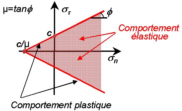
6.12.4. Operand ADHESION

Frictional stress at zero normal stress. Tensile strength is then given by:

\({R}_{T}=C/\mu\)

6.12.5. Operand AMOR_NOR

Normal damping surface density integrated on the surface of an element face 3D_JOINT then distributed as a discrete characteristic over each segment joining each pair of vertex nodes facing each other from one side of the element to the other. These characteristics are affected with their full value only if the joint element is in compression: or if the seventh internal variable component of behavior JOINT_MECA_FROT is negative.

So the unit is (in SI): PA.S.m-1

6.12.6. Operand AMOR_TAN

Tangential damping surface density integrated on the surface of an element face 3D_JOINT then distributed as a discrete characteristic over each segment joining each pair of vertex nodes facing each other from one side of the element to the other. These characteristics are affected with their full value only if the joint element is in compression: or if the seventh internal variable component of behavior JOINT_MECA_FROT is negative.

So the unit is (in SI): PA.S.m-1

6.12.7. Operand COEF_AMOR

If the joint element is not in compression when the seventh internal variable component of behavior JOINT_MECA_FROT is not negative, the previous normal or tangential damping characteristics are not affected with their full value but with a coefficient specified by the keyword COEF_NOR.

6.12.8. Operand PENA_TANG

Parameter for regularizing the sliding tangent matrix, is introduced to make the elementary tangent matrix invertible. By default, it is set to a value that is small in relation to the tangent stiffness. If the structure is subject to very significant slippage, it must be verified that the calculation is not sensitive to the value of this parameter.

6.12.9. Operand SCIAGE

The saw size used during the sawing phase. Only valid with mechanical joint models: xxx_ JOINT, and incompatible with RHO_FLUIDE, VISC_FLUIDE and OUV_MIN.

6.12.10. Operand PRES_FLUIDE

Pressure on the lips of the crack due to the presence of fluid (a function that may depend on geometric coordinates or the moment). Only valid with mechanical joint models: xxx_ JOINT, and incompatible with RHO_FLUIDE, VISC_FLUIDE and OUV_MIN.

6.12.11. Operand RHO_FLUIDE

Fluid density (positive real [mass]/[volume]), only valid for coupled hydro-mechanical models: xxx_ JOINT_HYME and incompatible with PRES_FLUIDE.

6.12.12. Operand VISC_FLUIDE

Dynamic viscosity of the fluid (strictly positive real in units of [pressure]). [time]), only valid for coupled hydro-mechanical models: xxx_ JOINT_HYME and incompatible with PRES_FLUIDE.

6.12.13. Operand OUV_MIN

Regularization aperture at the crack point (strictly positive real [length]), only valid for coupled hydro-mechanical models: xxx_ JOINT_HYME and incompatible with PRES_FLUIDE.

6.13. Keyword factor JOINT_MECA_ENDO

Law JOINT_MECA_ENDO is a unified behavior model for joints (main application for dams) [R7.01.25]. The latter makes it possible to model both the rupture and the friction between the lips of the joints. The surrounding material has pure mechanical behavior. Friction is managed by the internal plasticity variable and failure by the damage variable. The coupling takes place through the term kinematic work hardening. The law is written in the generalized standard formalism, it admits a hydro-mechanical coupling similar to that of the previous laws JOINT_MECA_FROT and JOINT_MECA_RUPT. The cleaving and sawing procedures are not activated.

6.13.1. K_N operand

Normal tensile stiffness.

6.13.2. K_T operand

Tangential stiffness.

6.13.3. MU operand

Coefficient of friction.

6.13.4. Bn operand

Pure tensile strength.

6.13.5. Bt operand

Pure shear strength.

6.13.6. Operand ALPHA

Initial damage parameter. This parameter makes it possible to extend the elastic zone in the damage zone to promote the transition between elastic and damaged zone if convergence difficulties are encountered. By default, a value of 1e-7 is recommended.

6.13.7. Operand PENA_RUPTURE

Regularization parameter in break.

6.13.8. Operand PRES_FLUIDE

Pressure on the lips of the crack due to the presence of fluid (a function that may depend on geometric coordinates or the moment). Only valid with mechanical joint models: xxx_ JOINT, and incompatible with RHO_FLUIDE, VISC_FLUIDE and OUV_MIN.

6.13.9. Operand RHO_FLUIDE

Fluid density (positive real [mass]/[volume]), only valid for coupled hydro-mechanical models: xxx_ JOINT_HYME and incompatible with PRES_FLUIDE.

6.13.10. Operand VISC_FLUIDE

Dynamic viscosity of the fluid (strictly positive real in units of [pressure]). [time]), only valid for coupled hydro-mechanical models: xxx_ JOINT_HYME and incompatible with PRES_FLUIDE.

6.13.11. Operand OUV_MIN

Regularization aperture at the crack point (strictly positive real [length]), only valid for coupled hydro-mechanical models: xxx_ JOINT_HYME and incompatible with PRES_FLUIDE.

6.14. Keyword factor CORR_ACIER

Law CORR_ACIER is a model of the behavior of steel, subject to corrosion in reinforced concrete structures. This model is developed in 1D and 3D elasto-plastic that is damaging to isotropic work hardening and is based on the Lemaître model, cf. [R7.01.20].

\(\{\begin{array}{c}\frac{{\sigma }_{\mathit{eq}}}{1-D}-R\left(p\right)-{\sigma }_{y}>0\hfill \\ \dot{{\epsilon }^{p}}=\frac{3}{2}\frac{\dot{\lambda }}{1-D}\frac{\stackrel{~}{\sigma }}{{\sigma }_{\mathit{eq}}}\\ \dot{r}=\dot{\lambda }=\dot{p}\left(1-D\right)\\ R={\mathit{kp}}^{1/m}\end{array}\). In the plastic field \(D=0\), otherwise \(D=\frac{\mathit{Dc}}{{p}_{R}-{p}_{D}}\left(p-{p}_{D}\right)\)

6.14.1. Operand D_CORR

Critical damage coefficient.

6.14.2. Operands ECRO_K, ECRO_M

Hardening law coefficients \(R={\mathrm{kp}}^{1/m}\).

6.14.3. SY operand

Initial elasticity limit, noted \({\sigma }_{y}\) in the equations.

6.15. Keyword factor ENDO_HETEROGENE

The characteristics of law ENDO_HETEROGENE, which is an isotropic damage model representing the formation and propagation of cracks, are described in [R5.03.24]. The presence of cracks in the structure is modelled by lines of broken elements (\(d\mathrm{=}1\)). The breakage of the elements can be caused either by the initiation of a new crack or by propagation. This law is adapted to heterogeneous materials (for example clay).

6.15.1. Operand WEIBULL

Parameter associated with the Weibull model.

6.15.2. SY operand

Initial elasticity limit, noted \({\sigma }_{y}\) in the equations.

6.15.3. Operand II

Tenacity \({K}_{\mathrm{IC}}\).

6.15.4. Operand EPAI

Thickness of the sample shown. Attention, if this value is purely geometric, it is necessary for this law of behavior.

6.15.5. GR operand

Seed from the random draw defining the initial defects. Allows you to obtain a unique result for each command file. If the seed is void, the draw will be truly random and will differ at each launch. By default, the value is 1.

6.16. Keyword factor RUPT_FM

Law RUPT_FMpermet to define the critical toughness of a material as a temperature-dependent criterion

6.16.1. Operand KIC

A temperature-dependent critical toughness function, generally expressed as \(\mathit{MPa}\sqrt{(m)}\). The user should pay attention to the consistency of the units used by this function. For example in SI units (\(\mathit{Pa}\), \(m\)) you will have to enter a function in \(\mathit{Pa}\sqrt{(m)}\), or for engineering units (\(\mathit{MPa}\), \(\mathit{mm}\)), you will have to enter a function in \(\mathit{MPa}\sqrt{(\mathit{mm})}\).

6.17. Keyword factor RUPT_TURON

Give the characteristics of the law of cohesive behavior CZM_TURON allowing to model the damage of a cracking interface with a coupling between the responses according to the different stress modes (opening mode N and tangent modes T1 and T2). In fact, the law makes it possible to consider different properties in normal and pure tangent modes (joint anisotropy). It is described in detail in the documentation [R7.02.21]. This law is typically used to model joints in structures made of composite materials such as wind turbine blades.

6.17.1. Operand GC_N

Critical surface energy density in pure normal mode translating to the energy cost of cracking in normal mode.

6.17.2. Operand GC_T

Critical surface energy density in pure tangential mode translating the energy cost of cracking in tangential mode.

6.17.3. Operand SIGM_C_N

Critical stress at break in pure normal mode.

6.17.4. Operand SIGM_C_T

Critical stress at break in pure tangential mode.

6.17.5. K operand

Initial stiffness of the interface, used as a penalty parameter.

6.17.6. Operand ETA_BK

Parameter \(\eta\) of the Benzeggagh-Kenane criterion.

6.17.7. Operand C_RUPT

A dimensionless parameter that defines « post-break » residual stiffness (when the element is completely damaged and the cohesive stress is zero) as a fraction of the initial stiffness. It is 0.001 by default and cannot exceed 0.1.

6.17.8. Operand CRIT_INIT

Parameter making it possible to choose the type of cut between modes giving the damage initiation criterion, among “YE” (elliptical criterion) or “TURON” (so-called Benzeggagh-Kenane criterion depending on the rate of mixing of the load).