9. Metallo-mechanical behaviors#

For metallurgical behavior (cf. [R4.04.01]), three laws of behavior are available: a characteristic law of metallurgical transformations of steel, of steel with tempering phases and a law characteristic of zirconium alloys.

Steel can comprise (at most) seven different metallurgical phases:

four cold phases (noted \(\alpha_\alpha\)) which are ferrite, pearlite, bainite And martensite
a hot phase, austenite (noted \(\gamma\))
two cold tempering phases for bainite and martensite

Zircaloy may comprise (at most) three different metallurgical phases:

Two cold phases: a pure phase \(\alpha\) and a mixed phase \(\alpha\)
A hot phase \(\beta\)

For mechanical behavior with the consideration of metallurgical transformations, he There are two models.

The first model (cf. [R4.04.02]) can be used for steel and for Zircaloy. We choose the desired material by activating, in the keyword factor COMPORTEMENT of non-linear operators, the RELATION_KIT keyword which is equal ACIER or ZIRC. The various relationships relating to this model are the same for these two materials (we treat the same phenomena) but the number of phases in presence is different.

The second model (see [R4.04.05]) is only available for Zircaloy (« RELATION_KIT =” ZIRC “``) and corresponds to the keyword META_LEMA_ANI under COMPORTEMENT.

9.1. Keyword factor META_ACIER#

Parameters to be filled in for steel metallurgy.

9.1.1. Parameters for phase changes#

TRC is a table-like concept produced by the operator [DEFI_TRC] and containing all the information provided by diagrams TRC (Transformation into Continuous cooling) of the steel in question.

AR3 is the quasistatic temperature at which the decomposition of austenite begins upon cooling.

note: It is necessary to be consistent between this value and that corresponding to the cooling curve. given by the [DEFI_TRC] command. Beyond a difference of 10°C, a An alarm will be issued and it is considered that the results may be false.

ALPHA is the \(\alpha\) coefficient of the Koïstinen-Marbürger law expressing the quantity of martensite formed as a function of temperature

\[{Z}_{\alpha_{m}}=1-\mathrm{exp}(\alpha ({M}_{s}-T))\]

MSO is the temperature at which \({M}_{s,0}\) martensitic transformation begins when this is total. In this case \({M}_{s}={M}_{s0}\).

AC1 is the quasistatic temperature at which the transformation into austenite begins upon heating.

AC3 is the quasistatic temperature at the end of transformation into austenite.

TAUX_1 is the value of the « delay » function (cf. [R4.04.01]) \(\tau_1(T)\) involved in the austenitic transformation model at temperature AC1.

TAUX_3 is the value of the « delay » function (cf. [R4.04.01]) \(\tau_3(T)\) involved in the austenitic transformation model at temperature AC3.

The change in the proportion of austenite is then defined by:

\[\dot{Z}=\frac{Z-{Z}_{\text{eq}}\left(T\right)}{\tau \left(T\right)}\]

with \({Z}_{\text{eq}}\left(T\right)\) which therefore has the shape of [Courbe].

_images/Forme1.gif — Fig. 9.1 Curve \({Z}_{\text{eq}}\left(T\right)\)#

and \(\tau \left(T\right)\) which has the shape of [Courbe].

_images/Forme2.gif — Fig. 9.2 Curve \(\tau \left(T\right)\)#

9.1.2. Grain size parameters#

The following four parameters cause the grain size calculation if they are entered:

\[\frac{d}{{dt}}(d)=\frac{1}{\lambda}\left (\frac{1}{d}-\frac{1}{{d}_{\text{lim}}} \right)\]

with \(\lambda ={\lambda }_{0}\cdot \exp \left(\frac{{Q}_{\text{app}}}{R T} \right )\) and \({d}_{\text{lim}}={d}_{\text{10}}\exp \left (-\frac{{W}_{\text{app}}}{R T} \right )\).

LAMBDA0 is the \({\lambda }_{0}\) material parameter

QSR_K is the activation energy parameter \(\frac{{Q}_{\text{app}}}{R T}\)

D10 is the \({d}_{\text{10}}\) material parameter

WSR_K is the activation energy parameter \(\frac{{W}_{\text{app}}}{R T}\)

9.2. Keyword factor META_ACIER_REVENU#

Parameters to be entered for steel metallurgy with its tempering phases.

9.2.1. Parameters for phase changes#

We consider a Johnson-Mehl-Avrami law to describe the evolution of the percentage of phase returned \({\tilde{Z}}^{r}_{\alpha_{\alpha}}\) according to the maintenance time \(t^{*}\) at a temperature \(T^{m}\) for both tempering phases (bainite and martensite).

\[{\tilde{Z}}^{r}_{\alpha_{\alpha}}(t^{*})=\left ( 1 - \exp\left\{ -b ({t^{*}})^n \right\} \right )\]

TEMP is the tempering temperature \(T^{r}\) and TEMP_MAINTIEN is the tempering temperature maintenance \(T^{m}\) involved in the identification of parameters.

BAINITE_B and BAINITE_N are the coefficients \(b\) and \(n\) for the case of bainite \({\alpha_{\alpha}}=b\).

MARTENSITE_B and MARTENSITE_N are the coefficients \(b\) and \(n\) for the case of martensite \({\alpha_{\alpha}}=m\).

9.3. Keyword factor META_ZIRC#

Parameters to be entered for Zircaloy metallurgy (cf. [R4.04.04]).

META_ZIRC = _F (
    ◆ TDEQ = float,
    ◆ N = float,
    ◆ K = float,
    ◆ T1C = float,
    ◆ T2C = float,
    ◆ AC = float,
    ◆ M = float,
    ◆ QSR_K = float,
    ◆ T1R = float,
    ◆ T2R = float,
    ◆ AR = float,
    ◆ BR = float,
)

Recall that the material contains two phases:

\(\alpha\): compact hexagonal cold phase
\(\beta\): centered cubic hot phase

TDEQ is the transformation start temperature \(\alpha \iff \beta\) at equilibrium.

N and K are material parameters relating to the model giving the proportion of \(\beta\) in a function of temperature, at equilibrium.

T1C is the transformation start temperature \(\alpha\) in \(\beta\) upon heating.

T2C is a material parameter used in calculating the start temperature of transformation \(\alpha\) into \(\beta\) upon heating.

AC and M are material parameters involved in the evolution model of \(\beta\) in heating.

T2R is a material parameter used in the calculation of the start temperature of transformation \(\beta\) to \(\alpha\) upon cooling.

AR and BR are material parameters involved in the evolution model of \(\beta\) to cooling.

QSR_K is the Arrhenius constant expressed in degrees Kelvin.

9.4. Keyword factor DURT_META#

Definition of characteristics relating to the calculation of hardness associated with steel metallurgy.

The hardness is calculated using a linear mixing law on the micro-hardness of the components:

The model is written \(H_{V}=\sum_{k}{Z}_{k}{H_{V}}_{k}\) with \(H_{V}\) the hardness (here) Vickers for example) of the polyphase point, \({Z}_{k}\) the proportion of the \(k\) phase and \({H_{V}}_{k}\) the hardness of phase \(k\).

F 1_DURT is the micro-hardness of the cold phase \(\mathrm{F1}\) (ferrite for steel).

F 2_DURT is the micro-hardness of the cold phase \(\mathrm{F2}\) (pearlite for steel).

F 3_DURT is the micro-hardness of the cold phase \(\mathrm{F3}\) (bainite for steel).

F 4_DURT is the micro-hardness of the cold phase \(\mathrm{F4}\) (martensite for steel).

C_DURT is the micro-hardness for the hot phase (austenite for steel).

F 3_REVENU_DURT is the micro-hardness of the cold tempered phase \(\mathrm{F3}\) (bainite for steel).

F 4_REVENU_DURT is the micro-hardness of the cold tempered phase \(\mathrm{F4}\) (martensite for steel).

9.5. Tags factor ELAS_META, ELAS_META_FO#

Definition of elastic characteristics, expansion and elastic limits for modeling a material undergoing metallurgical transformations (see [R4.04.02] or [R4.04.05]). These coefficients can either be constant with respect to temperature ELAS_META, or depend on temperature ELAS_META_FO (parameter “TEMP”).

Some coefficients depend on the metallurgical structure (parameter “META”).

Note:

With respect to model META_LEMA_ANI, thermal expansion is classically written without distinction of phases. Therefore, the keywords” C_ALPHA “,” PHASE_REFE “, and” “, and” EPSF_EPSC_TREF “are mandatory but not taken into account in the equations. Only the expansion coefficient “F_ALPHA” is considered.

This model is a law without a threshold so the elasticity limits and the law of mixtures are not useful.

Note:

Concerning the other models, for a steel, a maximum of 5 elasticity limits are entered, for Zircaloy, a maximum of three are entered.

9.5.1. Operands#

E = young

Young’s modulus, identical for all metallurgical phases.

NU = naked

Poisson’s ratio, identical for all metallurgical phases.

F_ALPHA = wrong

Average thermal expansion coefficient of cold phases.

C_ALPHA = callus

Average thermal expansion coefficient of the hot phase.

PHASE_REFE =/'CHAUD'
                   /'FROID'

Choice of the reference metallurgical phase (hot phase or cold phase).

In fact, to define zero thermal deformation, it is necessary to define the reference temperature \({T}_{\mathrm{ref}}\) (defined in AFFE_MATERIAU) and the reference metallurgical phase, so that the thermal deformation is considered zero at \({T}_{\mathrm{ref}}\) and in the reference metallurgical state.

EPSF_EPSC_TREF = delta

Deformation of the non-reference phase compared to the reference phase at temperature \({T}_{\mathrm{ref}}\): reflects the difference in compactness between face-centered cubic crystallographic structures (austenitic type) and centered cubic structures (ferritic type).

TEMP_DEF_ALPHA = TDA

Temperature in relation to which the expansion coefficient is defined. In case C_ALPHA is a function, this operand is mandatory.

PRECISION = eps

This real indicates how precisely a temperature \(T\) is close to the reference temperature (cf. [§3.1.4]).

F 1_SY = F1sy

Cold phase elasticity limit 1 for plastic behavior.

F 2_SY = F2sy

Cold phase elasticity limit 2 for plastic behavior.

F 3_SY = F3sy

Cold phase elasticity limit 3 for plastic behavior.

F 4_SY = F4sy

Cold phase elasticity limit 4 for plastic behavior.

C_SY = Fsy

Elastic limit of the hot phase for plastic behavior.

SY_MELANGE = f

Function used for the law of mixture on the elastic limit of multiphase material for plastic behavior.

:math:`{\sigma }_{y}=\left(1-f\left(z\right)\right){\sigma }_{y}^{\gamma }+f\left(z\right){\sigma }_{y}^{\alpha }`

F 1_S_VP = f1SVP

Cold phase elasticity limit 1 for viscous behavior.

F 2_S_VP = f2SVP

Cold phase elasticity limit 2 for viscous behavior.

F 3_S_VP = f3SVP

Cold phase elasticity limit 3 for viscous behavior.

F 4_S_VP = f4SVP

Cold phase elasticity limit 4 for viscous behavior.

C_S_VP = Please

Elastic limit of the hot phase for viscous behavior.

S_VP_MELANGE = Please

Function used for the mixing law on the elastic limit of multiphase material for viscous behavior.

:math:`{\sigma }_{c}=\left(1-f\left(z\right)\right){\sigma }_{c}^{\gamma }+f\left(z\right){\sigma }_{c}^{\alpha }`

9.6. Keyword factor META_ECRO_LINE#

Definition of five work hardening modules used in modeling the phenomenon of linear isotropic work hardening of a material undergoing metallurgical phase changes (see [R4.04.02]). These modules are temperature dependent.

9.6.1. Operands#

F 1_D_SIGM_EPSI = dsde1

Slope of the traction curve for the cold phase 1.

F 2_D_SIGM_EPSI = dsde2

Slope of the traction curve for the cold phase 2.

F 3_D_SIGM_EPSI = dsde3

Slope of the traction curve for the cold phase 3.

F 4_D_SIGM_EPSI = dsde4

Slope of the traction curve for the cold phase 4.

C_D_SIGM_EPSI = dsdec

Slope of the traction curve for the hot phase.

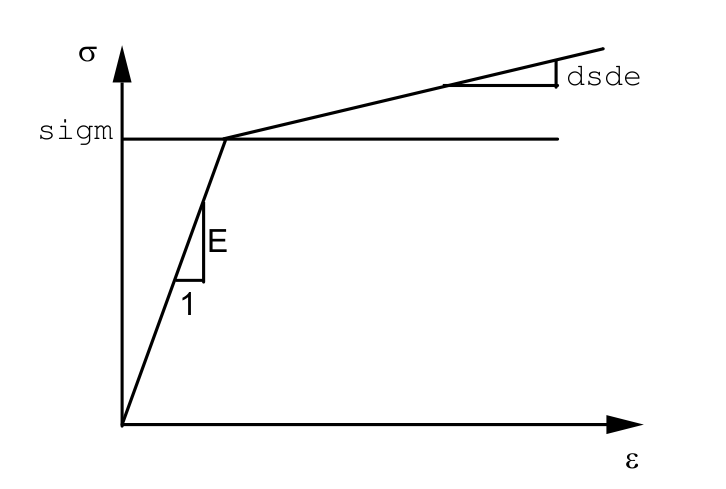
Young’s module \(E\) should be specified by the keywords META_ELAS or META_ELAS_FO.

9.7. Keyword factor META_TRACTION#

Definition of five tension curves used in modeling the phenomenon of non-linear isotropic work hardening of a material undergoing metallurgical phase changes (see [R4.04.02]). The traction curves may possibly depend on the temperature.

9.7.1. Operands#

SIGM_F1 = r_p1

Isotropic work hardening curve :math:`R` as a function of the cumulative plastic deformation :math:`p` for cold phase 1.

SIGM_F2 = r_p2

Isotropic work hardening curve :math:`R` as a function of the cumulative plastic deformation :math:`p` for the cold phase 2.

SIGM_F3 = r_p3

Isotropic work hardening curve :math:`R` as a function of the cumulative plastic deformation :math:`p` for the cold phase 3.

SIGM_F4 = r_p4

Isotropic work hardening curve :math:`R` as a function of the cumulative plastic deformation :math:`p` for the cold phase 4.

SIGM_C = r_p c

Isotropic work hardening curve :math:`R` as a function of the cumulative plastic deformation :math:`p` for the hot phase.

Note:

Attention this is not the curve \(\sigma\) function of \(\varepsilon\) but the curve \(R\) function of \(p\). We go from one to the other by performing the following calculations:

\(R=\sigma -\mathrm{limite}d’\mathrm{élasticité},p=\varepsilon –(\sigma /E)\mathrm{.}\)

9.8. Keyword factor META_VISC_FO#

Definition of the viscous parameters of the law of viscoplastic behavior taking into account metallurgy (see [R4.04.02]). The Norton-Hoff viscoplastic model has 5 parameters; the classical parameters \(\eta\), \(n\) of the power flow law, the elastic limit of viscous flow, the parameters \(C\) and \(m\) relating to the restoration of work-hardening of viscous origin. These parameters depend on the temperature and the metallurgical structure.

The elastic limit parameters are defined in ELAS_META.

9.8.1. Operands F 1_ETA /F 2_ETA /F 3_ETA /F 4_ETA/C_ETA#

F 1_ETA = eta1

Parameter \(\eta\) of the visco-plastic flow law, for the cold phase1.

F 2_ETA = eta2

Parameter \(\eta\) of the visco-plastic flow law, for the cold phase2.

F 3_ETA = eta3

Parameter \(\eta\) of the visco-plastic flow law, for the cold phase2.

F 4_ETA = eta4

Parameter \(\eta\) of the visco-plastic flow law, for the cold phase4.

C_ETA = etac

Parameter \(\eta\) of the visco-plastic flow law, for the hot phase.

9.8.2. Operands F1_N/F2_N/F3_N/F3_N/F4_N/C_N#

F1_N = n1

Parameter \(n\) of the visco-plastic flow law, for the cold phase 1.

F2_N = n2

Parameter \(n\) of the visco-plastic flow law, for the cold phase 2.

F3_N = n3

Parameter \(n\) of the visco-plastic flow law, for the cold phase 3.

F4_N = n4

Parameter \(n\) of the visco-plastic flow law, for the cold phase 4.

C_N = n5

Parameter n of the visco-plastic flow law, for the hot phase.

9.8.3. F1_C/F2_C/F3_C/F3_C/F4_C/C_C Operands#

F1_C = C1

Parameter \(C\) relating to the restoration of viscous work hardening, for the cold phase 1.

F2_C=C2

Parameter \(C\) relating to the restoration of viscous work hardening, for the cold phase 2.

F3_C = C3

Parameter \(C\) relating to the restoration of viscous work hardening, for the cold phase 3.

F4_C = C4

Parameter \(C\) relating to the restoration of viscous work hardening, for the cold phase 4.

C_C = C5

Parameter \(C\) relating to the restoration of viscous work hardening, for the hot phase.

9.8.4. Operands F1_M/F2_M/F3_M/F3_M/F4_M/C_M#

F1_M = m1

Parameter \(m\) relating to the restoration of viscous work hardening, for the cold phase 1.

F2_M = m2

Parameter \(m\) relating to the restoration of viscous work hardening, for the cold phase 2.

F3_M = m3

Parameter \(m\) relating to the restoration of viscous work hardening, for the cold phase 3.

F4_M = m4

Parameter \(m\) relating to the restoration of viscous work hardening, for the cold phase 4.

C_M = m5

Parameter \(m\) relating to the restoration of viscous work hardening, for the hot phase.

9.9. Keyword factor META_PT#

Definition of the characteristics used in modeling the transformation plasticity of a material that undergoes metallurgical phase changes (see [R4.04.02]).

The model is as follows: \(\Delta {\varepsilon }^{\mathrm{pt}}=\frac{3}{2}\sigma \sum _{i=1}^{i=4}{K}_{i}{F}_{i}^{\text{'}}({Z}_{i})\langle \Delta {Z}_{i}\rangle\)

9.9.1. Operands#

F1_K = Kf, F2_K = Kp, F3_K = Kb, F4_K = Km

Constants \({K}_{i}\) used in the transformation plasticity model, for the various cold phases. For steel = ferritic, pearlitic, bainitic and martensitic phase.

F 1_D_F_META =F'f, F 2_D_F_META =F'p, F 3_D_F_META =F'b, F 4_D_F_META =F'm,

Functions \({F}_{i}^{\text{'}}\) used in the transformation plasticity model, for the various cold phases. For steel: ferritic, pearlitic, bainitic and martensitic phases.

9.10. Keyword factor META_RE#

Definition of the characteristics used in modeling the phenomenon of work-hardening restoration of a material that undergoes metallurgical phase changes (see [R4.04.02]).

9.10.1. Operands#

C_F1_THETA =Tgf, C_F2_THETA =Tgp, C_F3_THETA =Tgb, C_F4_THETA =Tgm

Constants characterizing the rate of work hardening transmitted during the transformation of the hot phase C into the cold phase. For steel; transformation of austenite into ferrite, pearlite, bainite and martensite. Thus, \(\theta =0\) corresponds to a total restoration and \(\theta =1\) to a total transmission of work hardening.

F 1_C_THETA =Tfg, F 2_C_THETA =Tpg, F 3_C_THETA =Tbg, F 4_C_THETA =Tmg

Constants characterizing the rate of work hardening transmitted during the transformation of the cold phases into the hot phase. For steel; transformation of ferrite, pearlite, bainite, and martensite into austenite. Thus, \(\theta =0\) corresponds to a total restoration and \(\theta =1\) to a total transmission of work hardening.

9.11. Keyword META_LEMA_ANI#

Definition of the parameters of law META_LEMA_ANI (cf. [R4.04.05]), an elasto-viscous law without threshold with anisotropic behavior. Briefly, the model is written either in the cylindrical coordinate system \((r,\theta ,z)\), or in the Cartesian coordinate system \((\mathit{Ox},\mathit{Oy},\mathit{Oz})\):

Partition of deformations: \(\epsilon ={\epsilon }^{e}+\alpha \mathrm{\Delta }T\mathrm{Id}+{\epsilon }^{v}\)

Flow law of viscous deformation: \(\dot{{\epsilon }^{v}}=\dot{p}\frac{M\mathrm{:}\sigma }{{\sigma }_{\mathit{eq}}}\)

Hill criterion: \({\sigma }_{\mathit{eq}}=\sqrt{\sigma \mathrm{:}M\mathrm{:}\sigma }\)

Hill matrix \(\mathrm{M}\) in cylindrical coordinates:

\({\underline{M}}_{(r,\theta ,z)}=\left[\begin{array}{cccccc}{M}_{\mathit{rrrr}}& {M}_{\mathit{rr}\theta \theta }& {M}_{\mathit{rrzz}}& 0& 0& 0\\ {M}_{\mathit{rr}\theta \theta }& {M}_{\theta \theta \theta \theta }& {M}_{\theta \theta \mathit{zz}}& 0& 0& 0\\ {M}_{\mathit{rrzz}}& {M}_{\theta \theta \mathit{zz}}& {M}_{\mathit{zzzz}}& 0& 0& 0\\ 0& 0& 0& {M}_{r\theta r\theta }& 0& 0\\ 0& 0& 0& 0& {M}_{\mathit{rzrz}}& 0\\ 0& 0& 0& 0& 0& {M}_{\theta z\theta z}\end{array}\right]\)

\(\text{avec}\{\begin{array}{ccc}{M}_{\mathit{rrrr}}+{M}_{\mathit{rr}\theta \theta }+{M}_{\mathit{rrzz}}& \text{=}& 0\\ {M}_{\mathit{rr}\theta \theta }+{M}_{\theta \theta \theta \theta }+{M}_{\theta \theta \mathit{zz}}& \text{=}& 0\\ {M}_{\mathit{rrzz}}+{M}_{\theta \theta \mathit{zz}}+{M}_{\mathit{zzzz}}& \text{=}& 0\end{array}\)

or, in Cartesian coordinates:

\({\underline{M}}_{(x,y,z)}=\left[\begin{array}{cccccc}{M}_{\mathit{xxxx}}& {M}_{\mathit{xxyy}}& {M}_{\mathit{xxzz}}& 0& 0& 0\\ {M}_{\mathit{xxyy}}& {M}_{\mathit{yyyy}}& {M}_{\mathit{yyzz}}& 0& 0& 0\\ {M}_{\mathit{xxzz}}& {M}_{\mathit{yyzz}}& {M}_{\mathit{zzzz}}& 0& 0& 0\\ 0& 0& 0& {M}_{\mathit{xyxy}}& 0& 0\\ 0& 0& 0& 0& {M}_{\mathit{xzxz}}& 0\\ 0& 0& 0& 0& 0& {M}_{\mathit{yzyz}}\end{array}\right]\)

\(\text{avec}\{\begin{array}{ccc}{M}_{\mathit{xxxx}}+{M}_{\mathit{xxyy}}+{M}_{\mathit{xxzz}}& \text{=}& 0\\ {M}_{\mathit{xxyy}}+{M}_{\mathit{yyyy}}+{M}_{\mathit{yyzz}}& \text{=}& 0\\ {M}_{\mathit{xxzz}}+{M}_{\mathit{yyzz}}+{M}_{\mathit{zzzz}}& \text{=}& 0\end{array}\)

Law of mixtures on matrix \(\mathrm{M}\):

\(\begin{array}{c}M=\{\begin{array}{ccc}{M}^{c}& \text{si}& 0.00⩽{Z}_{f}⩽0.01\\ {M}^{2}={Z}_{f}{M}^{1}+(1-{Z}_{f}){M}^{c}& \text{si}& 0.01⩽{Z}_{f}⩽0.99\\ {M}^{1}& \text{si}& 0.99⩽{Z}_{f}⩽1.00\end{array}\\ {Z}_{f}={Z}_{1}+{Z}_{2};\text{}{Z}_{c}={Z}_{3}=1-{Z}_{f}\end{array}\)

Equivalent deformation rate: \(\dot{p}={\left(\frac{{\sigma }_{\mathit{eq}}}{{\mathit{ap}}^{m}}\right)}^{n}{e}^{-Q/T}\)

or equivalently: \({\mathrm{\sigma }}_{\mathit{eq}}=\underset{\text{contrainte visqueuse}{\mathrm{\sigma }}_{v}}{\underset{⏟}{a{\left({e}^{Q/T}\right)}^{1/n}{p}^{m}{\dot{p}}^{1/n}}}={\mathrm{\sigma }}_{v}\)

Law of mixtures on viscous stress \({\sigma }_{v}\):

\({\sigma }_{\mathit{eq}}={\sigma }_{v}=\sum _{i=1}^{3}{f}_{i}({Z}_{\alpha }){\sigma }_{\mathit{vi}}\) with \({\mathrm{\sigma }}_{\mathit{vi}}={a}_{i}{\left({e}^{{Q}_{i}/T}\right)}^{1/{n}_{i}}{p}^{{m}_{i}}{\dot{p}}^{1/{n}_{i}}\)

Note:

in the isotropic case, we have:

\(\begin{array}{}{M}_{\mathrm{rrrr}}={M}_{\theta \theta \theta \theta }={M}_{\mathrm{zzzz}}=1\\ {M}_{\mathrm{r\theta r\theta }}={M}_{\mathrm{rzrz}}={M}_{\theta z\theta z}=0.75\end{array}\)

\(\begin{array}{c}{M}_{\mathit{xxxx}}={M}_{\mathit{yyyy}}={M}_{\mathit{zzzz}}=1\\ {M}_{\mathit{xyxy}}={M}_{\mathit{xzxz}}={M}_{\mathit{yzyz}}=0.75\end{array}\)

The choice of the type of coordinates (cylindrical or Cartesian) is made respectively by detecting the keyword F_MRR_RR or the keyword F_MXX_XX.

9.11.1. Operands#

The table below summarizes the correspondence between the equation symbols and the keywords.

Symbol in equations	Key word
\(\mathrm{a1}\), \(\mathrm{a2}\), \(\mathrm{a3}\)	“F1_A”, “F2_A”, “C_A”
\(\mathrm{m1}\), \(\mathrm{m2}\), \(\mathrm{m3}\)	“F1_M”, “F2_M”, “C_M”
\(\mathrm{n1}\), \(\mathrm{n2}\), \(\mathrm{n3}\) :math:``	“F1_N”, “F2_N”, “C_N”
\(\mathrm{Q1}\), \(\mathrm{Q2}\), \(\mathrm{Q3}\)	“F1_Q”, “F2_Q”, “C_Q”

The Hill matrix is known either for the cold phase (1) “F_M**_**” or for the hot phase (3) “C_M**_**”.

Note:

The coefficients “F1_Q”, “F2_Q” and “C_Q “are in Kelvin degrees.