9. Keyword POUTRE#
9.1. Affordable characteristics#
This keyword makes it possible to assign the characteristics of the cross sections of beam elements (models POU_D_E, pou_d_em, POU_D_T, POU_D_TG, POU_D_TGM, POU_D_T_GD,, TUYAU_3M, TUYAU_6M).
We can treat several types of sections defined by the SECTION operand:
GENERALE: The mechanical characteristics are given.
RECTANGLE: The dimensions of the section are given. Code_Aster calculates the necessary mechanical characteristics: area, inertia,…
CERCLE: The dimensions of the section are given. Code_Aster calculates the necessary mechanical characteristics: area, inertia,…
COUDE: Used to define the inertia correction and stress amplification coefficients in the case where one wishes to take into account the ovalization of the section, which cannot be taken into account by the theory of beams. The mechanical characteristics are given by SECTION which can take the value GENERALE or RECTANGLE or CERCLE.
To each type of section, it is possible to assign different characteristics identified by one or more names (operand CARA) to which as many values are associated (operand VALE). It is also possible to give the characteristics via a table in the case of the general section, see the documentation for the macr_cara_girder command.
It is possible to treat beams with a constant cross section (characteristic name without suffix) or with a variable cross section (characteristic name with suffix 1 or 2). The mode of variation of the section is defined by the keyword VARI_SECT (cf. [§ 9.4.1]). The characteristics of the section are then given to the initial node (name with suffix 1) and to the final node (name with suffix 2) (« initial » and « final » relative to the numbering of the support mesh). This keyword should also be used to define the torsional constant for modeling (POU_D_EM).
9.2. Syntax#
POUTRE = _F (

♦ GROUP_MA = lgma, [l_gr_mesh]

**# general section**

**♦/SECTION** **= 'GENERALE',**

◊ VARI_SECT = ['CONSTANT', 'HOMOTHETIQUE'] [default]

# **constant general section**

/**♦** TABLE_CARA = tb_cara, [sd_table]

**♦** NOM_SEC = sec_name, [:ref:`K8 <K8>`]

/♦ CARA = |'A'|'IY'|'IY'|'IZ'|'IZ'|'AY'|'AZ'|'EZ',

|'JX'|'AI'|'RY'|'RY'|'RZ'|'RT',

|'JG'|'IYR2'|'IZR2',

♦ VALE = go, [l_real]

# **homothetic general section**

/♦ CARA = |'A1'|'A2'|'A2'|'IY1'|'IY2'|'IZ1'|'IZ2',

|'JX1'|'JX2'|'AY1'|'AY1'|'AY2'|'AZ1'|'AZ2',

| 'JG1'|'JG2'|'EY1'|'EY2'|'EY2'|'EZ1'|'EZ2',

|'RY1'|'RY2'|'RZ1'|'RZ2',

|'RT1'|'RT2'|'IYR21'|'IZR21',

| 'IYR22'|'IZR22',

♦ VALE = go, [l_real]

**# rectangle section**

**/ SECTION** **= 'RECTANGLE',**

◊ VARI_SECT = ['CONSTANT', 'HOMOTHETIQUE" AFFINE'], [default]

# **constant right section**

/♦ CARA =/|'H'|'EP',

/|'HY'|'HZ'|'EPY'|'EPZ',

♦ VALE = go, [l_real]

# **homothetic rectangle section**

/♦ CARA =/|'H1'|'H2'|'H2'|'EP1'|'EP2',

/|'HY1'|'HZ1'|'HY2'|'HZ2',

|'EPY1'|'EPY2'|'EPZ1'|'EPZ2',

♦ VALE = go, [l_real]

# **slim rectangle section**

/♦ CARA = |'HY'|'EPY'|'HZ1', |'EPZ1', |'EPZ1'|'HZ2'|'EPZ2',

♦ VALE = go, [l_real]

**# circle section**

**/ SECTION** **= 'CERCLE',**

◊ VARI_SECT = ['CONSTANT', 'HOMOTHETIQUE'], [default]

# **section** **constant circle**

/♦ CARA = |'R'|'EP',

♦ VALE = go, [l_real]

# **section** **homothetic circle on GROUP_MA**

/♦ CARA = |'R_DEBUT'|'R_END'|'EP_DEBUT'|'EP_FIN',

♦ VALE = go, [l_real]

**# elbow section**

**/ SECTION** **= 'COUDE',**

◊/◊ COEF_FLEX = cflex, [real]

/♦ COEF_FLEX_XY = cflex_xy, [real]

♦ COEF_FLEX_XZ = cflex_xz, [real]

◊/◊ INDI_SIGM = isigm, [real]

/♦ INDI_SIGM_XY = isigm_xy, [real]

♦ INDI_SIGM_XZ = isigm_xz, [real]

◊ MODI_METRIQUE = ['OUI', 'NON'], [default]

◊ TUYAU_NSEC = nsec (16), [integer (default)]

◊ TUYAU_NCOU = ncu (3), [integer (default)]

◊ FCX = fv, [function]

),
9.3. Rules of use#
Note:
The orientation of the beam elements is done by the keyword ORIENTATION [§ 10 ]. The twist angle (which makes it possible to orient the cross section of the beam around its neutral fiber) is always given to orient the main axes of the section, which is impractical, because these axes are generally unknown before calculating the geometric characteristics of the section, cf. MACR_CARA_POUTRE [U4.42.02] .
• It is possible to provide, via Python variables, the characteristics of the (general) sections resulting from a calculation with MACR_CARA_POUTRE (Cf. the test SSLL107F) .
• The various characteristic names of the operand arguments CARA are described later for each argument of the operand SECTION .
For a given mesh:
° You cannot overload one type of cross-section variation (constant or variable) by another.
° You cannot overload one type of section ( CERCLE , , RECTANGLE , GENERALE ) by another type of section ( * , ,). *
° For beams of variable cross section, names with suffix 1 or 2 are incompatible with names without a suffix. Example: \(A\) is incompatible with \(\mathit{A1}\) and \(\mathit{A2}\) .
◦ \(H\) is incompatible with \(\mathit{HZ}\) and \(\mathit{HY}\) (as well \(\mathit{H1}\) , \(\mathit{H2}\) ,…)
◦ \(\mathit{EP}\) is incompatible with \(\mathit{EPY}\) and \(\mathit{EPZ}\) (as well \(\mathit{EP1}\) , \(\mathit{EP2}\) ,…) .
◦ \(\mathit{RY}\) , \(\mathit{RZ}\) and \(\mathit{RT}\) are only used for the calculation of the constraints.
9.4. Operands#
9.4.1. Operand VARI_SECT#
Allows you to define the type of cross-section variation between the two end nodes of the beam element, elements POU_D_E and POU_D_T [R3.08.01].
The possibilities are:
Section |
Refine |
Homothetic |
circle |
no |
yes |
rectangle |
yes (next \(y\)) |
yes |
general |
no |
yes |
« Affine » means that the area of the section varies linearly between the two nodes. The dimensions in the y direction are constant (\(\mathit{HY}\), \(\mathit{EPY}\)) and the dimensions in the \(z\) direction vary linearly (\(\mathit{HZ1}\), \(\mathit{HZ2}\), \(\mathit{EPZ1}\), \(\mathit{EPZ2}\)).
« Homothetic » means that the dimensions of the section vary linearly between the values given at the two end nodes. In this case, the area of the section evolves quadratically.
In the case of circular hollow sections, for the section to be considered homothetic, it is necessary that \({\mathit{EP}}_{\mathit{DEBUT}}/{R}_{\mathit{DEBUT}}={\mathit{EP}}_{\mathit{FIN}}/{R}_{\mathit{FIN}}\). In the case of non-compliance with homothety the solution given by*Code_Aster* is approximated [R3.08.01].
9.4.2. Operand MODI_METRIQUE#
Allows you to define for elements TUYAU the type of integration in the thickness (models TUYAU_3M, TUYAU_6M):
MODI_METRIQUE = “NON” leads to the assimilation in integrations of the radius to the mean radius. This is therefore valid for pipes of small thickness (relative to the radius),
MODI_METRIQUE = “OUI” implies complete integration, which is more precise for thick pipes, but which can in some cases lead to oscillations in the solution.
9.4.3. Operand SECTION = “GENERALE”#
9.4.3.1. Constant section#
In this specific case, the section characteristics can be given by the keywords table_cara and nom_sec instead of cara and vale. You can also give TABLE_CARA a table from the macro-command macr_cara_poutreby entering in the NOM_SEC keyword:
the name of the mesh given to macr_cara_girder, if the section corresponds to the whole mesh.
the name of the group of elements to which the section corresponds.
You can also give it a table from the read_table operator. To do this, the table must be defined as follows:
NOM_SEC |
A |
IY |
IZ |
AY |
AZ |
|
SEC_1 |
a1 |
iy1 |
iy1 |
iz1 |
ay1 |
az1 |
SEC_2 |
a2 |
iy2 |
iy2 |
iz2 |
ay2 |
az1 |
Column names are the names of the characteristics in the section. If a column contains non-real values (except in column NOM_SEC), it will be ignored. If the name of a column is not in the list of possible characteristics it will be ignored.
In this case sec_name can take the value \({\mathit{sec}}_{1}\) or \({\mathit{sec}}_{2}\).
9.4.3.2. Homothetic section#
The characteristics are defined for each stitch, at the two nodes.
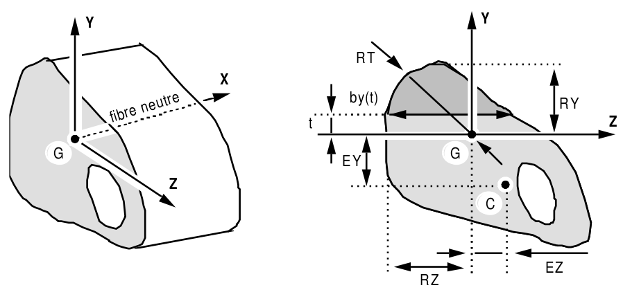
Figure 9.4.3.2-1: Section GENERALE.
Definition of characteristics:
\(\mathit{IZ}=\underset{s}{\int }{y}^{2}\mathit{ds}\) |
|
\(\mathit{AY}=\frac{A}{{A}_{y}^{\text{'}}}=\frac{A}{{\mathit{IZ}}^{2}}\underset{{y}_{1}}{\overset{{y}_{2}}{\int }}\frac{{m}_{y}^{2}(y)}{{b}_{y}(y)}\mathit{dy}\) |
|
with \({m}_{y}(y)=\underset{y}{\overset{{R}_{y}}{\int }}{\mathit{t.b}}_{y}(t)\mathit{dt}\) \({b}_{y}(t)\) thickness following \(z\), in \(z\mathrm{=}t\) |
\({b}_{z}(t)\) thickness following \(y\), in \(y\mathrm{=}t\) |
With:
\({A}_{y}^{\text{'}}\), \({A}_{z}^{\text{'}}\): reduced sheared areas.
\({A}_{y}^{\text{'}}\mathrm{=}\frac{A}{\mathit{AY}}\) with \(\mathrm{AY}\ge 1\) or even \({A}_{y}^{\text{'}}\mathrm{=}{k}_{y}A\) with \({k}_{y}=\frac{1}{\mathit{AY}}\le 1\)
shear coefficients \({A}_{y},{A}_{z}\) are used by elements POU_D_T, and POU_D_TG, POU_D_TGM, for the calculation of stiffness and mass matrices and for the calculation of stresses [R3.08.01]. In particular, transverse shear stresses are expressed by:
\({\tau }_{\mathit{xz}}=\frac{{V}_{z}}{{K}_{z}A}={V}_{z}\frac{{A}_{z}}{A}\) \({\tau }_{\mathit{xy}}={V}_{y}\frac{{A}_{y}}{A}\)
in the case of Euler beams (POU_D_E) that do not take into account transverse shear, the corresponding terms are neglected in the calculation of stiffness and mass by taking \({A}_{y}={A}_{z}=0\). On the other hand, shear stresses [R3.08.01] are calculated by:
\({\tau }_{\mathrm{xz}}=\frac{{V}_{z}}{A}\) \({\tau }_{\mathrm{xy}}=\frac{{V}_{y}}{A}\)
Characteristics \(\mathrm{RY}\), \(\mathrm{RZ}\), \(\mathrm{RT}\) are used to calculate flexural and torsional stresses [R3.08.01] for the options” SIGM_ELNO “or” SIPO_ELNO “of CALC_CHAMP [U4.81.04].
Flexing \({\sigma }_{\mathit{xx}}=\frac{{M}_{y}}{{I}_{y}}.\mathit{RZ}-\frac{{M}_{z}}{{I}_{z}}.\mathit{RY}\)
Twisting \({\tau }_{\mathit{xz}}={\tau }_{\mathit{xy}}=\frac{\mathit{MT}}{\mathit{JX}}.\mathit{RT}\)
9.4.4. Operand SECTION = “RECTANGLE”#
CARA |
Significance |
Default values |
Constant section |
||
HY |
Dimension of the next rectangle \(\mathrm{GY}\) |
Mandatory |
HZ |
Dimension of the next rectangle \(\mathrm{GZ}\) |
Mandatory |
HHHH |
Square dimension (if the rectangle is square) |
Mandatory |
EPY |
Thickness next \(\mathrm{GY}\) in the case of a hollow tube |
HY/2 |
EPZ |
Thickness next \(\mathrm{GZ}\) in the case of a hollow tube |
HZ/2 |
EP |
Thickness along both axes in the case of a hollow tube |
Full tube |
Homothetic section |
||
H1, H2 |
Dimension of the square at each end for a variable cross section |
H1= H2= H |
HY1, HY2 |
Dimension of the next rectangle \(\mathrm{GY}\) at each end for a variable cross section |
HY1 = HY2 = HY |
HZ1, HZ2 |
Dimension of the next rectangle \(\mathrm{GZ}\) at each end for a variable cross section |
HZ1 = HZ2 = HZ |
EP1, EP2 |
Thickness along both axes in the case of a hollow tube, at each end in the case of a variable section |
EP1 = EP2 = EP |
EPY1, EPY2 |
Thickness next \(\mathrm{GY}\) in the case of a hollow tube, at each end in the case of a variable cross section |
EPY1 = EPY2 = EPY |
EPZ1, EPZ2 |
Thickness next \(\mathrm{GZ}\) in the case of a hollow tube, at each end in the case of a variable cross section |
EPZ1 = EPZ2 = EPZ |
In the case of rectangular hollow sections, the homothetic can only be in the direction \(y\) [R3.08.01].
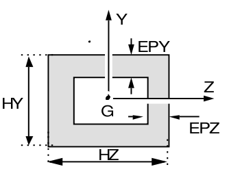
Figure 9.4.4-1: Section RECTANGLE.
The characteristics calculated by*Code_Aster* are [R3.08.03]:
\(\mathit{Iy}=\frac{\mathit{HY}{\mathit{HZ}}^{3}}{12}-\frac{(\mathit{HY}-2\mathit{EPY}).{(\mathit{HZ}-2\mathit{EPZ})}^{3}}{12}\) \(\mathrm{RY}=\frac{\mathrm{HY}}{2}\)
\(\mathit{Iz}=\frac{\mathit{HZ}{\mathit{HY}}^{3}}{12}-\frac{(\mathit{HZ}-2\mathit{EPZ}){(\mathit{HY}-2\mathit{EPY})}^{3}}{12}\) \(\mathrm{RZ}=\frac{\mathrm{HZ}}{2}\)
If the tube is hollow:
\(\mathrm{JX}=\frac{\mathrm{2.EPY.EPZ}{(\mathrm{HY}-\mathrm{EPY})}^{2}{(\mathrm{HZ}-\mathrm{EPZ})}^{2}}{\mathrm{HY.EPY}+\mathrm{HZ.EPZ}-{\mathrm{EPY}}^{2}-{\mathrm{EPZ}}^{2}}\)
\(\mathit{RT}=\frac{\mathit{JX}}{2\mathit{EPZ}(\mathit{HY}-\mathit{EPY})(\mathit{HZ}-\mathit{EPZ})}\)
If the tube is full, install:
\(\begin{array}{c}a=\frac{\mathit{HY}}{2},b=\frac{\mathit{HZ}}{2}\mathit{si}\mathit{HY}>\mathit{HZ}\\ a=\frac{\mathit{HZ}}{2},b=\frac{\mathit{HY}}{2}\mathit{si}\mathit{HZ}>\mathit{HY}\end{array}\) \(J=a{b}^{3}\left(\frac{16}{3}-3.36\frac{b}{a}+0.28\frac{{b}^{5}}{{a}^{5}}\right)\)
\(\mathit{RT}=\frac{J\left(3a+1.8b\right)}{8{a}^{2}{b}^{2}}\)
Shear coefficients \(\mathit{Ay}\) and \(\mathit{Az}\)
We pose \({\alpha }_{y}=\frac{\mathit{HY}-2\mathit{EPY}}{\mathit{HY}}\) \({\alpha }_{z}=\frac{\mathit{HZ}-2\mathit{EPZ}}{\mathit{HZ}}\)
The values for \(\mathit{AY}\) and \(\mathit{AZ}\) are given by the table below: Tab (column, row)
\(\mathit{AY}=\mathit{Tab}({\alpha }_{y},{\alpha }_{z})\) \(\mathit{AZ}=\mathit{Tab}({\alpha }_{z},{\alpha }_{y})\)
Tab |
0.00 |
0.05 |
0.05 |
0.10 |
0.30 |
0.40 |
0.50 |
0.50 |
0.60 |
0.60 |
0.60 |
0.60 |
0.60 |
0.60 |
0.60 |
0.60 |
0.60 |
0.60 |
0.95 |
||
0.00 |
1.200 |
1.200 |
1.200 |
1.200 |
1.200 |
1.200 |
1.200 |
1.200 |
1.200 |
1.200 |
1.200 |
1.200 |
1.200 |
||||||||
0.05 |
1.200 |
1.209 |
1.209 |
1.209 |
1.212 |
1.212 |
1.212 |
1.212 |
1.212 |
1.212 |
1.207 |
1.207 |
1.202 |
1.201 |
|||||||
0.10 |
1.200 |
1.229 |
1.229 |
1.229 |
1.236 |
1.236 |
1.253 |
1.241 |
1.241 |
1.230 |
1.230 |
1.230 |
1.230 |
1.217 |
1.217 |
1.206 |
1.202 |
||||
0.20 |
1.200 |
1.300 |
1.300 |
1.300 |
1.317 |
1.339 |
1.348 |
1.332 |
1.309 |
1.309 |
1.309 |
1.280 |
1.280 |
1.280 |
1.280 |
1.247 |
1.247 |
1.247 |
1.217 |
1.206 |
|
0.30 |
1.200 |
1.413 |
1.413 |
1.413 |
1.442 |
1.477 |
1.479 |
1.451 |
1.408 |
1.408 |
1.354 |
1.354 |
1.354 |
1.354 |
1.295 |
1.295 |
1.295 |
1.295 |
1.238 |
1.214 |
|
0.40 |
1.200 |
1.577 |
1.577 |
1.621 |
1.621 |
1.671 |
1.662 |
1.614 |
1.545 |
1.45 |
1.460 |
1.460 |
1.460 |
1.460 |
1.460 |
1.460 |
1.366 |
1.366 |
1.272 |
1.230 |
|
0.50 |
1.200 |
1.803 |
1.803 |
1.803 |
1.866 |
1.936 |
1.913 |
1.838 |
1.733 |
1.608 |
1.608 |
1.608 |
1.608 |
1.608 |
1.608 |
1.608 |
1.608 |
1.608 |
1.469 |
1.469 |
1.325 |
0.60 |
1.200 |
2.115 |
2.115 |
2.207 |
2.207 |
2.309 |
2.267 |
2.154 |
2.000 |
1.818 |
1.818 |
1.818 |
1.619 |
1.619 |
1.409 |
1.301 |
|||||
0.70 |
1.200 |
2.561 |
2.561 |
2.561 |
2.704 |
2.894 |
2.640 |
2.409 |
2.409 |
2.140 |
2.140 |
2.140 |
2.140 |
1.848 |
1.848 |
1.541 |
1.378 |
||||
0.80 |
1.200 |
3.265 |
3.265 |
3.265 |
3.520 |
3.830 |
3.90 |
3.524 |
3.154 |
2.154 |
2.720 |
2.720 |
2.720 |
2.252 |
2.252 |
1.771 |
1.517 |
||||
0.90 |
1.200 |
4.715 |
4.715 |
5.358 |
5.358 |
6.536 |
6.401 |
5.916 |
5.186 |
4.186 |
4.300 |
4.300 |
4.300 |
3.300 |
3.331 |
3.331 |
2.338 |
1.841 |
|||
0.95 |
1.200 |
6.689 |
6.689 |
8.194 |
10.294 |
11.236 |
11.189 |
10.375 |
9.014 |
7.296 |
7.296 |
7.296 |
7.296 |
5.296 |
5.372 |
5.372 |
3.367 |
2.371 |
Remarks:
• The values in the table are determined using a parametric study carried out with the command macr_cara_beam.
• The interpolations on the values in the table are linear.
• For values of \(\alpha >0.95\) , the user must calculate the shear coefficient values himself.
• Calculated values can be printed with the keyword * INFO = 2.
9.4.5. Operand SECTION = “CERCLE”#
CARA |
Significance |
Default value |
Constant section |
||
RRRR |
Outer radius of the tube |
Mandatory |
EP |
Thickness in the case of a hollow tube |
Solid tube (EP=R) |
Variable section assigned on a mesh |
||
R1, R2 |
External radii at both ends for a variable cross section |
R1= R2= R |
EP1, EP2 |
Thicknesses at both ends in the case of a variable cross section. |
EP1 = EP2 = EP |
Variable section assigned to a mesh group |
||
R_DEBUT, R_FIN |
External radii at both ends of the beam defined by the group of elements |
None |
EP_DEBUT, EP_FIN |
Thicknesses at both ends of the beam defined by the group of elements |
None |
In the case of a variable section assigned to a group of elements, the characteristics are automatically calculated from the values at the ends. To do this, the cells must be correctly oriented and contiguous in the group.
In the case of circular hollow sections, for the section to be homothetic you need \(\mathit{EP1}/\mathit{R1}=\mathit{EP2}/\mathit{R2}\). In the case of non-compliance with this condition the solution given by Code_Aster is approximated [R3.08.01], an alarm message is sent to warn the user.
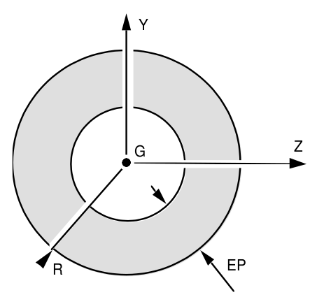
Figure 9.4.5-1: Section CERCLE.
The values calculated by*Aster* are [R3.08.03]: \(\begin{array}{c}{I}_{y}={I}_{z}=\frac{\mathit{JX}}{2}=\frac{\pi {R}^{4}}{4}-\frac{\pi {(R-\mathit{EP})}^{4}}{4}\\ \mathit{RT}=\mathit{RY}=\mathit{RZ}=R\end{array}\)
Shear coefficients \(\mathit{Ay}=\mathit{Az}\). with \(\alpha =\frac{R-\mathit{EP}}{R}\)
Notes:
• The values in the table are determined using a parametric study carried out with the command macr_cara_beam.
• Interpolations are linear.
• Calculated values can be printed with the keyword * INFO = 2.
9.4.6. Operand SECTION = “COUDE”#
When one wishes to take into account flexibility correction coefficients or stress amplification coefficients, the modeling of the bends must be done by modeling POU_D_T. To obtain correct results, it is recommended to model a 90° elbow with 20 to 40 POU_D_T meshes. Characteristics are only assignable on elements POU_D_T.
The assignment of mechanical characteristics (section, inertia,…) is carried out by SECTION which can take the value GENERALE or RECTANGLE or CERCLE.
9.4.6.1. Operand COEF_FLEX, COEF_FLEX_XZ, COEF_FLEX_XY: flexibility coefficients#
◊ coef_flex= \(\mathrm{cflex}\)
◊ coef_flex_xz = \({\mathrm{cflex}}_{\mathrm{xz}}\)
◊ coef_flex_xy = \({\mathrm{cflex}}_{\mathrm{xy}}\)
For the modeling of pipe bends, the representation by elements of a circular beam is insufficient to represent the flexibility of a thin shell. The flexibility coefficient adjusts the geometric data (geometric moments of inertia) in accordance with construction rules. Certain rules lead to the calculation of flexural stiffness with a corrected geometric moment of inertia:
\({I}_{y,z}=\frac{{I}_{y,z}(\mathrm{tube})}{\mathrm{cflex}}\) with \(\mathrm{cflex}>1.0\)
A classic value of \(\mathrm{cflex}\), for pipes with a thickness \(e\) and an average radius \({R}_{\mathrm{moy}}\), is given by:
\(\mathrm{cflex}=\frac{1.65}{\lambda }\) with \(\lambda =\frac{e{R}_{\mathrm{courb}}}{{R}_{\mathrm{moy}}^{2}}\)
This value can be calculated directly in the command file, see for example test FORMA01A [V7.15.100].
In the case where 2 coefficients are given, we get: \({I}_{y}=\frac{{I}_{y}(\mathit{tube})}{{\mathit{cflex}}_{\mathit{xy}}},{I}_{z}=\frac{{I}_{z}(\mathit{tube})}{{\mathit{cflex}}_{\mathit{xz}}}\)
By default, \(\mathit{cflex}={\mathit{cflex}}_{\mathit{xz}}={\mathit{cflex}}_{\mathit{xy}}=1\) (no change in geometric inertia).
Note: \({\mathit{cflex}}_{\mathit{xy}}\) is applied to \({I}_{y}\) , , \({\mathit{cfle}}_{\mathit{xz}}\) is applied to \({I}_{z}\) .
9.4.6.2. Operands INDI_SIGM, INDI_SIGM_XZ, INDI_SIGM_XY: Intensification of constraints#
◊ INDI_SIGM = \(\mathrm{isigm}\)
◊ INDI_SIGM_XZ = \({\mathrm{isigm}}_{\mathrm{xz}}\)
◊ INDI_SIGM_XY = \({\mathrm{isigm}}_{\mathrm{xy}}\)
For the calculation of the flexural stresses in the elements of tubular cross-section beams, it is possible to take into account an intensification coefficient due to ovalization. The constraints are then written as:
\({\sigma }_{\mathit{xx}}\mathrm{=}\frac{{M}_{y}\mathrm{.}R}{{I}_{y}}\mathrm{\times }\mathit{isigm}\) or \({\sigma }_{\mathit{xx}}\mathrm{=}\frac{{M}_{z}\mathrm{.}R}{{I}_{z}}\mathrm{\times }\mathit{isigm}\) with \(\mathit{isgim}\mathrm{\ge }1\)
In the case where 2 indices are given, we have:
\({\sigma }_{\mathit{xx}}=\frac{{M}_{y}.R}{{I}_{y}}\times {\mathit{isigm}}_{\mathit{xy}}\) or \({\sigma }_{\mathit{xx}}=\frac{{M}_{z}.R}{{I}_{z}}\times {\mathit{isigm}}_{\mathit{xz}}\)
By default, \(\mathit{isigm}={\mathit{isigm}}_{\mathit{xz}}={\mathit{isigm}}_{\mathit{xy}}=1\) (no change in geometric inertia).
Note: \({\mathit{isigm}}_{\mathit{xy}}\) is applied to \({M}_{y}\) , , \({\mathit{isigm}}_{\mathit{xz}}\) is applied to \({M}_{z}\) .
9.5. Operand FCX#
◊ FCx = fv
Assignment of a function describing the dependence of the distributed force on the relative wind speed (see test SSNL118 [V6.02.118]). Wind loading is applicable on cable bar and beam elements (models POU_D_E, POU_D_T, POU_D_TG, POU_D_T_GD, POU_D_TGM).
9.6. Operands TUYAU_NSEC/TUYAU_NCOU#
◊ TUYAU_NSEC = nsec (16) [integer (default)]
◊ TUYAU_NCOU = ncu (3) [integer (default)]
Number of layers in the thickness (ncu, by default 3) and sectors (nsec, by default 16) on the circumference used for integrations in elements TUYAU [R3.08.06]. The values by default (3 layers and 16 sectors) correspond to a minimum required for correct precision.