2. Synthesis of cohesive models#

2.1. Theoretical framework#

The cohesive models presented here are based on the variational approach to rupture proposed by Frankfurt and Marigo [bib2]. Based on a principle of energy minimization, it makes it possible to represent the initiation and propagation of cracks, without a priory hypothesis about their space-time evolution and regardless of the load applied. This theory postulates that the equilibrium configuration of a structure is one that minimizes, at each loading increment, its total energy, the sum of potential energy and surface energy. The latter corresponds to the energy dissipated to create one or more cracks.

The numerical models proposed here are limited to the search for a state of equilibrium (or satisfying the equations of motion in dynamics) of a structure for which the potential cracking path is known beforehand.

2.2. Finite element models#

In Code_Aster, there are three types of finite elements designed to model cracking with a cohesive law. The first two presented below are classically used in literature (see [bib5] or [bib6]), the third is innovative and makes it possible to combine the advantages of the previous two even if, for the moment, it remains under validation.

The classic joint element ( \(\mathrm{EJ}\) ), arranged along potential cracks, makes it possible to discretize the displacement jump with an order in accordance with the other elements of the mesh. On the other hand, it requires a regularization of the cohesive law by penalizing the conditions of contact and adherence, apparently a source of instabilities in the overall response of the structure. In addition, it leads to spatial oscillations of cohesive forces that may prove to be unacceptable, due to their collocation at the Gauss points of the elements.

Models: PLAN_JOINT, AXIS_JOINT, 3D_ JOINT

Documentation: [R3.06.09] and [U3.13.14]

The discontinuity element ( \(\mathrm{ED}\) ) included discretizes both the movement jump (constant per piece) and the surrounding volume displacement field (\(\mathrm{Q1}\)). It fulfills its objective, which is to take into account the conditions of adherence without regularization. On the other hand, contrary to what was expected, the geometric position of the crack is not left free, unless it deviates from an energetic formulation. In addition, its limitation to elastic behavior in a semi-static state and the insufficient order of discretization make it limited in practice.

Modelings: PLAN_ELDI, AXIS_ELDI

Documentation: [R7.02.14] and [U3.13.14]

More recently, the development of a third family of finite elements has made it possible to reconcile the advantages of the previous two. Also arranged along potential cracks, the mixed interface element ( \(\mathrm{EI}\) ****) ** provides a discretization of the displacement field (\(\mathit{P2}\)), the cohesive forces (\(\mathrm{P1}\)) and the displacement jump (\(\mathit{P1}\) -discontinuous or \(\mathit{P2}\) -discontinuous). In this way:

it allows the treatment of adhesion conditions without any regularization, resulting in more regular structural responses;
it respects condition LBB which guarantees satisfactory convergence with mesh refinement, with the same rate as for volume elements (quadratic convergence);
it is compatible with any law of volume behavior.
on the other hand it is only compatible with a quadratic mesh

For interface elements, a distinction is made between standard modeling *_ INTERFACE and sub-integrated modeling*_ INTERFACE_S. In the first, the displacement jump is modelled by a \(\mathit{P2}\) -discontinuous field, while in the second it is modeled by a \(\mathit{P1}\) -discontinuous field. Each of these models has advantages and disadvantages. Standard modeling limits the risk of zero pivots appearing in the tangent matrix, but does not strictly verify condition LBB. To remedy this, it is recommended to choose an augmented Lagrangian penalty parameter that is not too large (this choice provides a bit of « flexibility » in modeling). Sub-integrated modeling better verifies condition LBB, but more often has zero pivots in the tangent matrix. These pivots appear in particular when the interface is located on a plane of symmetry, or between a volume and a structural element (MEMBRANE, GRILLE or BARRE).

The first applications confirm the potential of this element, which will have succeeded in synthesizing the two previous families. Its application in dynamics to treat sudden propagations is planned in the short term.

Models: PLAN_INTERFACE, AXIS_INTERFACE, 3D_ INTERFACE, PLAN_INTERFACE_S,, AXIS_INTERFACE_S, 3D_ INTERFACE_S

Documentation: [R3.06.13] and [U3.13.14]

Finished element template	\(\mathrm{EJ}\)	\(\mathrm{ED}\)	\(\mathrm{EI}\)
Mechanical problem	Minimum energy	Minimum energy	Minimum energy under constraints
Modeling	2D plane, axis and 3D	2D plane, axis	2D plane, axis and 3D
Dimension finite elements	Surface	Surface	Volume	Surface
Type of elements	QUAD4, HEXA8, PENTA6	QUAD4	QUAD8, HEXA20, PENTA15
Form of energy	Regularized	Unregulated	Unregulated
Surrounding material	Linear or Nonlinear	Linear	Linear or Nonlinear	Linear or Nonlinear
Interpolation	Displacement P1, Jump P1	Displacement P1, Jump P0	Displacement P2, Constraints P1, Jump P1 Discontinuous or P2 Discontinuous
Influence of numerical parameters	Great influence of the numerical parameter	Great influence of the numerical parameter	Weak influence of the numerical parameter
Type of calculations	Statics and dynamics	Statics	Statics and dynamics (?)

Table 1: summary of the advantages and limitations of the finite element models mentioned above.

In table 1 we find the advantages of models \(\mathrm{EJ}\) and \(\mathrm{ED}\) in the model \(\mathrm{EI}\) without having the limits: non-regularized law, linear or non-linear material behavior, jump \(\mathrm{P1}\) and numerical parameter that does not influence the results of the calculation, while this is the case with that of \(\mathrm{EJ}\).

2.3. Cohesive laws#

Cohesive laws are a relationship between the stress vector and the displacement jump at each gauss point. All of these laws are non-linear and should be used with the nonlinear operators STAT/DYNA_NON_LINE (therefore they are not suitable for MECA_STATIQUE). For the previous models the cohesive laws are called:

EJ: CZM_LIN_REG, CZM_EXP_REG

ED: CZM_EXP

EI: CZM_OUV_MIX, CZM_TAC_MIX, CZM_EXP_MIX CZM_FAT_MIX, CZM_TRA_MIX, CZM_LAB_MIX

An example, in open mode (Figure 2.3), is given of the relationship between the normal component of the stress vector \({\sigma }_{n}\) and the normal jump \({\delta }_{n}\). The internal variable threshold \(\kappa\) makes it possible to manage the irreversibility of the cracking. The mechanical parameters of the law are the critical priming stress \({\sigma }_{c}\) and the critical energy release rate \({G}_{c}\). The ratio of these two parameters defines a critical jump \({\delta }_{c}={\mathrm{2G}}_{c}/{\sigma }_{c}\) beyond which the constraint is cancelled.

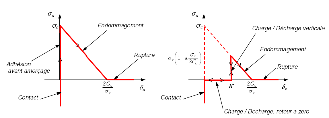
Figure 2.3:Normal component of the stress vector as a function of the normal jump for law CZM_OUV_MIX (threshold \(\kappa\) zero on the left and positive on the right).

The main differences between laws CZM relate to the priming phase and the form of the post-peak law. REG laws take into account the contact/membership part in a penalized manner while the others carry out these phases in a perfect manner (infinite slope at the origin, see figure 2.3). Note that the regularization of cohesive laws has an influence on the results of the calculation (see part 15). Moreover, the EXP laws (except CZM_EXP_MIX whose law was deliberately truncated) have an exponential decreasing behavior that tends asymptotically towards zero with the opening of the lips. Formally, these do not make it possible to define a crack tip; we will prefer the other linear decay laws which explicitly provide the position of the crack bottom (critical rupture jump, see figure 2.3).

In general, during the crack propagation phase, the shape of the cohesive law (linear or exponential) has little influence on the cracking, on the other hand, it can have a role on the initiation phase. For more details on these laws see [R7.02.11].

2.4. Definition of the local coordinate system at the crack#

For the integration of the cohesive law that involves a displacement jump, a function of the nodal displacements expressed in the global coordinate system, it is necessary to know a local coordinate system \((n,\mathrm{t1},\mathrm{t2})\) to the element. For EIs and EJ two different methods have been selected, each with its advantages but also its limitations.

For \(\mathrm{EI}\) : the user provides the information necessary to define the local coordinate system (in 2D, a rotation angle is sufficient, in 3D you need to know the three nautical angles). It is relatively simple for a straight or flat crack. It gets a lot more complex when that’s no longer the case. On the other hand, this method makes it possible to impose a single local coordinate system on all the elements of a given plane crack and thus allows a coherent visualization of the movement jumps in \(\mathrm{II}\) and \(\mathrm{III}\) modes. We’ll see that this is not the case for \(\mathrm{EJ}\) and \(\mathrm{ED}\).

For an interface mesh group FISS in a given plane, the user enters the characteristics of the EIs in the following manner (nautical angles \((a,b,c)\) in degrees):

ORIEN_FI = AFFE_CARA_ELEM (

MODELE =ME,

MASSIF =(

_F (GROUP_MA =” FISS “, ANGL_REP =( a, b, c)),

));

then CARA_ELEM = ORIEN_FI in STAT_NON_LINE.

In 2D it is easy to know the angle between the normal of the local coordinate system \(n\) and the vector \(X\) of the global coordinate system. This angle is the first nautical angle, the other two are set to zero. In 3D it’s a bit more difficult. To help the user we provide some examples of nautical angles with the definition of the local coordinate system \((n,\mathrm{t1},\mathrm{t2})\) in the global coordinate system \((X,Y,Z)\).

\((0,0,0):(n,\mathrm{t1},\mathrm{t2})=(X,Y,Z)\)

\((90,0,0):(n,\mathrm{t1},\mathrm{t2})=(Y,-X,Z)\)

\((-90,0,-90):(n,\mathrm{t1},\mathrm{t2})=(-Y,-Z,X)\)

\((0,-90,-90):(n,\mathrm{t1},\mathrm{t2})=(Z,X,Y)\)

For the \(\mathrm{EJ}\) and \(\mathrm{ED}\): The local coordinate system is calculated (hard) from the geometric coordinates of the element. No information is given by the user, taking into account cracks that are not rectilinear or not flat is therefore immediate. On the other hand, for a plane crack, the elements all have the same normal but tangent vectors \((\mathrm{t1},\mathrm{t2})\) that are different from one element to another. This of course has no impact on the validity of the calculations, but it prevents a clean visualization of the components of the jump in \(\mathrm{II}\) or \(\mathrm{III}\) mode.