4. Tips for use#
Cohesive models cover a fairly broad spectrum of use in the field of fracture mechanics. We start the user tips with general information on the use of parameters and on loads, valid regardless of the type of simulation. We continue by giving specific advice for brittle fracture calculations (linear or non-linear material), fatigue calculations and dynamic calculations. Subsequently, the importance of relying on numerical tools to improve the convergence of calculations is emphasized. Finally, we end with advice for post-processing the results.
4.1. Generalities#
4.1.1. Mechanical parameters#
The mechanical parameters of the law are the critical priming stress \({\sigma }_{c}\) and the critical energy release rate \({G}_{c}\). In Figure 2.3 on the left, the constraint \({\sigma }_{c}\) corresponds to the peak of the law, the density \({G}_{c}\) is related to the area under the triangle. The user defines a material and (non-zero) values of these parameters under the keyword RUPT_FRAG. In the case of thermal loading, it is possible to make them depend on temperature. In this case, the keyword RUPT_FRAG_FO is used, see example in the SDNS105a test.
The ratio of these two parameters defines a critical jump \({\delta }_{c}={\mathrm{2G}}_{c}/{\sigma }_{c}\) beyond which the constraint is cancelled for laws CZM_LIN_REG, CZM_OUV_MIX, CZM_TAC_MIX. For both laws CZM_EXP_REGet CZM_EXPla constraint tends asymptotically towards zero. For law CZM_EXP_MIX, a critical jump is defined at \({\delta }_{c}={\mathrm{3.2G}}_{c}/{\sigma }_{c}\). This jump corresponds to an error in the critical energy return rate of 1%. For fatigue law CZM_FAT_MIX, the jump value in clear of which the stress remains zero depends on the load. For ductile law CZM_TRA_MIX the shape parameters provided by the user influence this critical leap. For more details see the documentation [R7.02.11].
Note :
When imposing symmetry conditions on the lips of the crack it may be necessary to divide the value of \({G}_{c}\) by two, see part 16.
4.1.2. Numeric parameters#
Elements with internal discontinuity: There are no numerical parameters to enter for this model.
Joint element: This model has two numerical parameters intended to penalize adhesion PENA_ADHERENCE and contact PENA_CONTACT. We replace the parts that are infinitely rigid (contact and adhesion) by highly rigid elastic contributions (see doc [R7.02.11]). By default PENA_CONTACT is 1 and leads to a penalty identical to that of adherence, this is the recommended value. The parameter PENA_ADHERENCE corresponds to a percentage of the internal length of the cohesive law; it must be non-zero and less than 1. The lower the value, the greater the penalty slope.
The calculation results are highly dependent on the value of this parameter. In general, we observe:
Oscillations (local snapbacks) in the overall response of the structure linked to the successive opening of the joints. But also oscillations in the stress profile along the crack, which are all the more marked as the stiffness of the joint is important.
An important influence of the parameter on the quality of the solution under stress. For fairly low values of PENA_ADHERENCE the error is reasonable, for higher values it can lead to very large differences.
The convergence of the global Newton algorithm is all the more difficult as the penalization is important.
Therefore, antagonistic effects of the penalization parameter are observed, which involve making a compromise between convergence of the calculation and the precision of the solution. It is therefore difficult to recommend a general rule providing the right value for this parameter. It is therefore recommended to perform a sensitivity test to this parameter before carrying out a numerical simulation. In all cases, the initial stiffness of the joint elements must be greater than the stiffness of the neighboring solid elements.
Interface element: This model has a numerical parameter PENA_LAGR which corresponds to the penalization of the augmented Lagrangian (see [R3.06.13]). The calculation results do not depend on the value of this parameter. It is recommended to take the value by default (100). This value must be strictly greater than 1 in order to ensure the uniqueness of the solution during the integration of the cohesive law.
Moreover, laws CZM_OUV_MIX and CZM_TRA_MIXdestinées when opening in mode I only have a parameter called RIGI_GLIS which makes it possible to impose non-zero stiffness when sliding and thus avoid zero pivot problems when the elements break. We recommend using the default value of 10. The solution is not affected by this setting as long as the sliding modes are not enabled.
4.1.3. Loads and boundary conditions#
All types of mechanical and thermal loads can be a priori applied to a structure comprising cohesive elements: imposed displacements, surface forces, volume forces, temperature fields resulting from a prior thermal calculation.
To save on calculation time, taking into account the symmetries of the problem, it is often useful to simulate a semi-structure. Symmetry conditions on the lips of the cohesive crack (i.e. the faces of the cohesive elements), leading to an opening in pure I mode, can be envisaged in two different ways:
The first consists in blocking the normal movements of the faces of the cohesive elements that are not connected to the volume. The latter then coincide with the axis of symmetry of the structure. In this case, care should be taken with respect to the value of the critical surface energy density entered by the user. Since we are only modeling a crack lip, for a given material value of \({G}_{c}\), we must enter G_C= \({G}_{c}/2\) in the command file. In other words, it costs half as much energy to open a half-crack.
The second is to have the crack open completely. Symmetric movements with respect to an axis passing between them are imposed on the lips of the crack (command AFFE_CHAR_MECA/LIAISON_GROUP). This type of modeling makes it possible to take into account the crack as a whole and does not require the step of dividing \({G}_{c}\) by two. On the other hand, this poses a problem on the energy balance since we model a semi-structure (therefore a volume energy that is twice less) with a complete crack. This method should therefore be used very carefully; it is recommended to adopt the previous one instead.
4.1.4. Convergence criterion#
The convergence criterion of Newton’s algorithm RESI_REFE_RELA makes it possible to build a reference nodal force, which is used to estimate the (approximate) nullity of the residue (see [R5.03.01]). This makes it possible to improve convergence in the case where the residues are heterogeneous, that is to say when different degrees of freedom are treated. This is the case of the mixed EI model for which the use of this criterion is recommended.
With cohesive models, force is defined based on a constraint and its dual displacement. To use this criterion, we therefore enter a constraint and a reference displacement: SIGM_REFE and DEPL_REFE. To choose these values, we propose those from the cohesive law: the priming constraint \({\sigma }_{c}\) for the first, and the characteristic length \({G}_{c}/{\sigma }_{c}\) for the second. With the EJ and ED models it is not possible (and a priori not useful) to use this type of residue.
4.1.5. Linear solver#
The method for solving the global linear system MUMPS is essential for mixed elements with Lagrange-type degrees of freedom. It is therefore necessary to use it with EIs. Its main advantage lies in its ability to rotate rows and/or columns of the matrix during factorization in case of a small pivot. The other finite element models EJ and ED do not have this restriction; they can be used with the method by default (multifrontal).
Moreover, the tangent matrix of cohesive laws is symmetric; the use of the keyword SYME =” OUI “intended to symmetrize the latter is not necessary.
4.2. A linear interface to validate your data entry#
In the same way that it is recommended to perform a linear elastic calculation prior to a plastic calculation, it is preferable to start a cracking calculation by using a linear cohesive behavior relationship. The CZM_ELAS_MIX model was introduced for this purpose, see [U4.51.11]. This makes it possible to validate its data layout (orientation of the interfaces, numbering of the degrees of freedom, numbering of the degrees of freedom, assignment of characteristics and loads, etc.) in a framework simple enough for mechanical intuition (or the failure of the calculation) to be sufficient to detect possible outlier results.Attention, however: this behavioral relationship is only available with interface elements (EI).
This interface model is elastic, with one stiffness in the normal direction and another in both tangent directions. They are defined via DEFI_MATERIAU [U4.43.01] under the keyword factor CZM_ELAS. It is also possible to consider limiting behaviors via perfect normal and/or tangential grip conditions, always under the same keyword factor (in this case, stiffness no longer plays a role since the jump in movement in the normal or tangent direction is forced to zero). Typically, with perfect adhesion conditions (normal and tangential), the response of the structure must be very close to that which it would have without an interface (very close but not necessarily equal due to the mixed formulation used with the element EI).
Finally, a final adhesion condition is proposed: these are contact conditions when closed, accompanied by elastic stiffness when opened. The calculation becomes more complex because the problem is no longer linear. But this makes it possible to ensure that the areas where the interface opens and those where it remains closed are in accordance with intuition.
4.3. Fragile fracture calculations#
Possible models: EJ, EI, Recommended Model: EI
Cohesive models are suitable for modeling brittle failure in linear (all) or non-linear (EJ and EI only) material. One gives here some advice specific to this type of simulation. Numerical tools make it possible to guarantee the good robustness of the resolution algorithms, and advice on their use is also provided.
4.3.1. Linear material#
For a linear elastic material, there are no specific implementation precautions other than the previous generalities (part 15) and that on the mesh (part 9). For the robustness of the calculations, the use of load control is essential. Below is a section devoted to tips for using this method.
4.3.2. Nonlinear material#
The cohesive EJ and EI models can interact with any surrounding nonlinear material a priori. The possible simulations remain in the field of brittle fracture in the presence of plasticity, which is confined to the vicinity of the crack point. No specific numerical processing is necessary for this type of calculation, except for the usual precautions on the fineness of the mesh (see part 9) in order to capture the cohesive zone but also the plastic band along the lips of the crack. The convergence of the Newton-Raphson algorithm is slowed down (more Newton iterations at a given loading step) and the calculation time is increased but this remains entirely reasonable and does not hinder the robustness of cohesive models in this field of application.
From a mechanical point of view, the plasticization of the material as well as cracking are two phenomena that interact. Thus, particular attention should be paid in choosing the ratio of the initiation stress of the cohesive law and the elastic limit of the material.
Depending on the values of these parameters, we may find ourselves either in the case where cracking occurs without the development of plasticity, or in the opposite case where the stress in the material reaches the plastic threshold and evolves without exceeding the priming stress, or finally the case where plasticity and cracking evolve together. In the latter case, a plastic zone is observed that initiates at the crack point and evolves with the propagation of the crack.
In addition, some calculations with viscoplastic materials have been carried out for illustrative purposes; the poor feedback in this field does not allow us to provide specific advice.
4.3.3. Digital tools#
Linear search
It is possible to use linear search with cohesive models. This can occasionally improve the convergence of calculations. However, this method is not the best suited for overcoming the instabilities associated with the sudden propagation of cracks in a semi-static manner. In this case, loading control will be preferred.
Load control
Load control, available for all cohesive models, makes it possible to ensure the convergence of the Newton-Raphson algorithm into a semi-static state despite instability in the overall response of the structure (sudden crack propagation for example). This method is valid for softening laws that can lead to this type of response and in particular for cohesive laws. The idea is to allow the load to be relaxed in order to return some of the potential energy and to advance the cracking progressively by locally controlling the damage to the cohesive zones.
The user provides the direction of the load (displacement or surface force) from a AFFE_CHAR_MECA, this is multiplied by the scalar control parameter \(\eta\), a new unknown of the problem which gives its intensity. This last parameter replaces the multiplicative load function FONC_MULT. When solving the mechanical problem, an additional equation (pilot control) is added that closes the system. For more details on this technique, the reader can refer to the general documentation [R5.03.80] and to the specific piloting documentation for cohesive models [R7.02.11] and [R7.02.14].
This digital tool is particularly important to ensure the convergence of the algorithm. It is often necessary, even when the overall response does not allow for a step back. Indeed, in certain configurations, local setbacks, linked to a sudden opening at the elementary level, may occur. All cohesive laws can be controlled by elastic prediction (PRED_ELAS), the ratio of the time step \(\Delta t\) to the coefficient COEF_MULT makes it possible to manage the evolution of cracking. At the level of the law of behavior, this is equivalent to controlling the exit from the threshold. The higher this ratio is, the more quickly you want to get through the instability and therefore the higher \(\eta\) will be.
In the command STAT_NON_LINE, we choose to control the load TRACTION (entered classically) in the following way:
EXCIT = _F (CHARGE = TRACTION, TYPE_CHARGE = 'FIXE_PILO'),


The data specific to piloting are then added:


PILOTAGE = _F (

SELECTION = 'RESIDU',

TYPE = 'PRED_ELAS',

GROUP_MA = 'JOINT',

COEF_MULT = c_mult_pilo,

),
Notes and advice:
It is recommended to define the direction of the load*driven by a unit vector. Thus, the control parameter* \(\eta\) will correspond exactly to its intensity.
The user is advised to start by choosing u n report \(\Delta t\) out COEF_MULT equal to 0.05. In this way, the aim is to damage the most stressed Gauss point by 5%.
If the algorithm does not converge despite the piloting, it is advisable to reduce the previous ratio: under automatic or manual step cutting and/or increasing by COEF_MULT . The lower the ratio, the slower the cracking will be and vice versa.
It is sometimes*necessary to break the symmetry of the problem to avoid the pilot oscillating between two values of* \(\eta\) if these provide an identical state of cracking. To do this, it is recommended to perform a first non-linear calculation with a very low uncontrolled loading step. We thus remain in the d linear domain of the response and the calculation converges quickly.
Another way to avoid oscillations in the control value consists in entering a ETA_PILO_R_MIN equal to zero in order to allow only positive values of the control parameter.
It is necessary to finely control (low criterion output) the first controlled loading steps in order to correctly capture the peak value of the global response.
If the piloting is used in a case where it could be avoided, the solution is not modified. The only difference is that the intensity of the load is not directly controlled.
It is not*possible to control thermal loads.*
4.4. Ductile fracture calculations#
Possible models: EI
Law CZM_TRA_MIX was introduced in version 10.4 to try to model ductile breakage. The use of it must be limited to an initial research framework. Indeed, it is currently being validated and will certainly be subject to change.
The law for ductile rupture is inspired by the laws classically proposed in the literature. In addition to the parameters of critical stress and critical energy density, two parameters related to the shape of the law are added (COEF_EXTR and COEF_PLAS). The latter is chosen to be trapezoidal. Parameter sensitivity calculations as well as tests on CT (SSNP151) and AE (SSNA120) specimens were carried out. The first conclusions show that this model makes it possible to correctly reproduce the global response and the propagation kinetics observed with a Gurson (Rousselier) model on a 2D CT (SSNP151a). However, it should be noted that the adjustment of the parameters of the law to approach the fine calculation of the local approach remains difficult. On the other hand, the gain in calculation time and robustness is significant. When using a 3D CT (SSNP151b), the results are less conclusive after a certain level of loading. It seems that this is partly due to the poor consideration of volume effects in the cohesive model and in particular the confinement effect. Work is in progress to try to take into account the influence of triaxiality. Other limitations should also be emphasized: as for other cohesive models, the crack path must be known a priori. Cracking can only take place in mode I (it is however possible to introduce sliding modes if this proves to be appropriate). Finally, large crack openings are not taken into account; however, it is possible to use large deformations in the surrounding material.
No specific numerical processing is necessary for this type of calculation, except for the usual precautions on the fineness of the mesh (see part 9) in order to capture the cohesive zone but also the plastic band along the lips of the crack. The convergence of the Newton Raphson algorithm is slowed down (more Newton iterations at a given loading step) and the calculation time is increased but this remains entirely reasonable and does not hinder the robustness of cohesive models in this field of application.
From a mechanical point of view, the plasticization of the material as well as cracking are two phenomena that interact. Thus, particular attention should be paid in choosing the ratio of the initiation stress of the cohesive law and the elastic limit of the material. Depending on the values of these parameters, we may find ourselves either in the case where cracking occurs without the development of plasticity, or in the opposite case where the stress in the material reaches the plastic threshold and evolves without exceeding the priming stress, or finally the case where plasticity and cracking evolve together. In the latter case, a plastic zone is observed that initiates at the crack point and evolves with the propagation of the crack.
4.4.1. Digital tools#
Linear search
It is possible to use linear search. This can occasionally improve the convergence of calculations.
Load control
It is considered that cracks propagate progressively in ductile failure mode. Cargo control is therefore not developed for this type of law.
4.5. Fatigue calculations#
Possible model: \(\mathrm{EI}\)
The law available to deal with the fatigue phenomenon in \(I\) mode is CZM_FAT_MIX (see doc [R7.02.11]) usable with interface elements. Calculations can be carried out in 2D or 3D regardless of the material and for all types of mechanical loads (of constant or variable amplitude), or thermal loads. We can also refer to tests SSNP118JKL and SSNP139B and to part 25.
To account for fatigue with this law, it is necessary to go through all the loading cycles. It is easy to understand that it is not possible to simulate a large number of cycles. However, the first results highlight a certain number of phenomena observed in fatigue (see report [bib3]). For elastic material:
We manage to reproduce Paris-type laws of evolution whose coefficients are identified*a posteriori,
We note the slight influence of overload on progress,
The absence of a sequence effect with variable amplitude is observed,
Realistic 3D crack front evolutions are simulated.
In the presence of plasticity, several effects observed experimentally are reproduced:
We highlight the overload effect which leads to the slowdown of propagation due to the compression induced by the increase in the plastic zone,
the slowdown is all the more pronounced the greater the overload,
The increase in the load ratio contributes to reducing the delay at a fixed overload ratio and load amplitude.
In addition, work on the skipping of cycles is envisaged. By extrapolation, they will make it possible to simulate a large number of cycles.
Advice on discretizing loading:
When discretizing cyclic loading, some precautions should be taken to optimize the calculation time. The risk is to perform an automatic redistribution of the step at each cycle, which can become very expensive in CPU. The feedback allows us to advise the user to perform approximately 4 loading increments per cycle when the material is elastic and to double this value when this one behaves non-linear. This rule is not necessarily valid in all situations and will have to be adapted on a case-by-case basis to optimize the time spent in each cycle.
Advice on the definition of the cyclical function:
To build the multiplicative load function you can use DEFI_FONCTION or python in the commandfile. An example of a sawtooth function with variable amplitude is given below. The odd times are the ends of increase in charge (amplitude max) and the even moments are the ends of discharge (amplitude min). In this way, we complete the \(i\) th cycle at instant \(\mathrm{2i}\). In the example below the load varies
From val_inf*to* val_sup*during cycles 1 to* nb_cy_1,
From val_inf*to* val_surch*during cycles* nb_cy_1+1 to nb_cy_2,
From val_inf*to* val_sup*during cycles* nb_cy_2+1 and nb_cy_3
Example of a cyclic function f with variable amplitude:
f = []
for i in xrange (nb_cy_1):
f.extend ((2*i, val_inf,2*i+1, val_sup))
for i in range (nb_cy_1, nb_cy_2):
f.extend ((2*i, val_inf,2*i+1, val_surch))
for i in range (nb_cy_2, nb_cy_3):
f.extend ((2*i, val_inf,2*i+1, val_sup))
The definition of the function concept in Code_Aster is then carried out classically:
FCT_FAT = DEFI_FONCTION (
NOM_PARA = “INST”,
PROL_GAUCHE =” LINEAIRE “,
VALE = f,
)
Advice on data storage
To avoid*storing too large databases, we recommend keeping only the values of the fields at the top of each cycle using the keyword* ARCHIVAGE de STAT_NON_LINE . To do this, it is of course necessary to discretize the load that passes through the vertices.
4.6. Dynamic calculations#
Possible models: \(\mathrm{EJ}\), \(\mathrm{EI}\) (under validation), Recommended template: \(\mathrm{EJ}\)
Taking dynamic aspects into account introduces additional complexity into modeling. In addition to the precautions for use in quasistatics (mesh refinement sufficient to discretize the cohesive zone, which is relatively small for the characteristics of steels (of the order of 1 mm)), the dynamic regime imposes additional rules. We offer the following few practical tips based on feedback. You can also refer to the [bib1] report.
First of all, the integration diagram: the Newmark diagram called « of mean acceleration (\(d=1/2\), \(a=1/4\)) (,), unconditionally stable and non-dissipative in a linear environment, seems the best suited (no numerical dissipation detected in the presence of cohesive zones). Very few tests have been tested with other schemes (explicit, Wilson…) but have led to convergence problems. A thesis is in progress (D. Doyen) to optimize patterns in the presence of shocks.
As far as time discretization is concerned, everything depends on the phenomena we are trying to simulate. To precisely identify the reflections of the waves on the cohesive zone (causing a disturbance in the kinematics of the crack), it is necessary (always for the usual characteristics of steels) to consider time steps less than or equal to \({10}^{\text{-}8}s\). If a coarser follow-up of the kinematics is sufficient and the important phenomenon is priming and stopping, then steps of the order of \({10}^{\text{-}7}\le \Delta t\le {10}^{\text{-}5}s\) are sufficient. Above, convergence problems appear (\(\Delta t\approx {10}^{\text{-}6}s\) seems to be a good compromise).
Particular attention must be paid to the transition from a stable phase to an unstable phase (more precisely a phase where the cohesive zone extends progressively, then where it spreads abruptly). In this case, the time steps must be adapted to capture the moment when the cohesive zone accelerates, otherwise the « dynamic effect » will be completely erased. The use of load control in a near static manner, combined with the observation of the snapback of the global response can provide information on this critical moment.
The small parameter PENA_ADHERENCE representing the stiffness of the joint before decohesion (regularization parameter) must be taken less than \({10}^{\text{-}4}\). In fact, below this value the results are no longer sensitive to this parameter.
In general, feedback is limited in this field of application. The use of these models in dynamics remains, for the moment, intended for specialists.
4.7. Post-treatment of cracking and control POST_CZM_FISS#
Visualization of cracking for \(\mathrm{EJ}\) and \(\mathrm{EI}\)
To visualize a cohesive crack, several solutions are possible:
The internal variable at the gauss point (VARI_ELGA) :math:`mathrm{V3}` is a**crack indicator* that allows you to know if the gauss point is healthy (\(\mathrm{V3}=0\)), damaged (\(\mathrm{V3}=1\)), or broken (\(\mathrm{V3}=2\)). See example figure 4.5.
Variable :math:`mathrm{V4}` varies continuously from 0 (healthy) to 1 (broken); it corresponds to the**percentage of surface energy dissipated* and can be interpreted as an indicator of damage. See example figure 4.5.
You can also visualize the values of the* jump of displacement** in the three break modes I, II and III respectively using the internal variables \(\mathrm{V7}\), \(\mathrm{V8}\) and \(\mathrm{V9}\).
A**dissipation indicator* \(\mathrm{V2}\) allows you to know if the Gauss point is dissipating energy or is in unloads (the values taken by this internal variable depend on the cohesive law, see doc [R7.02.11]).
Finally, we can visualize the components of the cohesive force in the three rupture modes \(I\), \(\mathrm{II}\) and \(\mathrm{III}\) respectively using the stress vector at the Gauss point SIEF_ELGA: SIGN, SITXet SITY. The sign of SIGNpermet to know if the point is in contact or not.
Attention, for \(\mathrm{EJ}\) the visualization of tangential jumps in \(\mathrm{II}\) and \(\mathrm{III}\) mode (respectively \(\mathrm{V8}\) and \(\mathrm{V9}\)) does not make sense given that the tangential vectors of the local coordinate system are independent from one element to another (see part 7 on this subject).
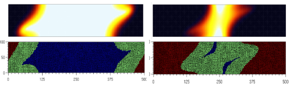
Figure 4.5 : Evolution of the fracture in mixed mode in a 3D beam, visualization of the crack plane.
Internal variable \(\mathrm{V4}\) at the top (1 in black, 0 in white) and \(\mathrm{V3}\) at the bottom (0 in blue, 1 in green, 2 in red).
Visualization of cracking for EDs
For \(\mathrm{ED}\) the internal variables are not the same, the percentage of energy dissipated is stored in \(\mathrm{V5}\) and the dissipation indicator in the variable \(\mathrm{V4}\). We also store the normal and tangential stresses in \(\mathrm{V6}\) and V7 as well as the jumps in normal and tangential displacement in \(\mathrm{V1}\) and \(\mathrm{V2}\).
POST_CZM_FISS : calculating the length of cohesive cracks in 2D
This command makes it possible to know, at each moment, the size of the cohesive crack as well as the size of the cohesive zone from the coordinates of a point POINT_ORIG and a direction vector VECT_TANG given by the user. The latter must also enter the result of the non-linear evol_noli calculation as well as the group of cohesive elements grma on which he wishes to perform post-processing. The syntax is as follows:
table_saster = POST_CZM_FISS (RESULTAT = evol_noli,
GROUP_MA = Grma,
POINT_ORIG = (R, R),
VECT_TANG =( R, R))
This command can be used for models PLAN_JOINT, PLAN_INTERFACE, AXIS_JOINT and AXIS_INTERFACE and for cohesive laws CZM_OUV_MIX, CZM_TAC_MIX, CZM_LIN_REG, CZM_EXP_REG. The crack lengths are evaluated based on the geometric position of the Gauss points and the internal variable V3 of the cohesive laws which makes it possible to know the state of the point (healthy, damaged, broken). Refer to the POST_CZM_FISS U4 documentation for more information. An example of use is provided in the ssnop139a and ssnop139c tests.
Crack length calculation in 3D
It is possible to extend the macro above for 3D but this is not planned in the short term.