3. Tips on meshing#
After some generalities on the different types of finite elements, advice is provided on the creation of the mesh as well as on its characteristics in order to correctly model the cohesive crack in various configurations.
3.1. Generalities#
In general, cohesive models make it possible to represent a crack on a given \(\Gamma\) path a priori. These models account for evolution but not for the direction of propagation. It is therefore necessary to produce a mesh compatible with the potential crack path. It consists in arranging cohesive elements along this path.
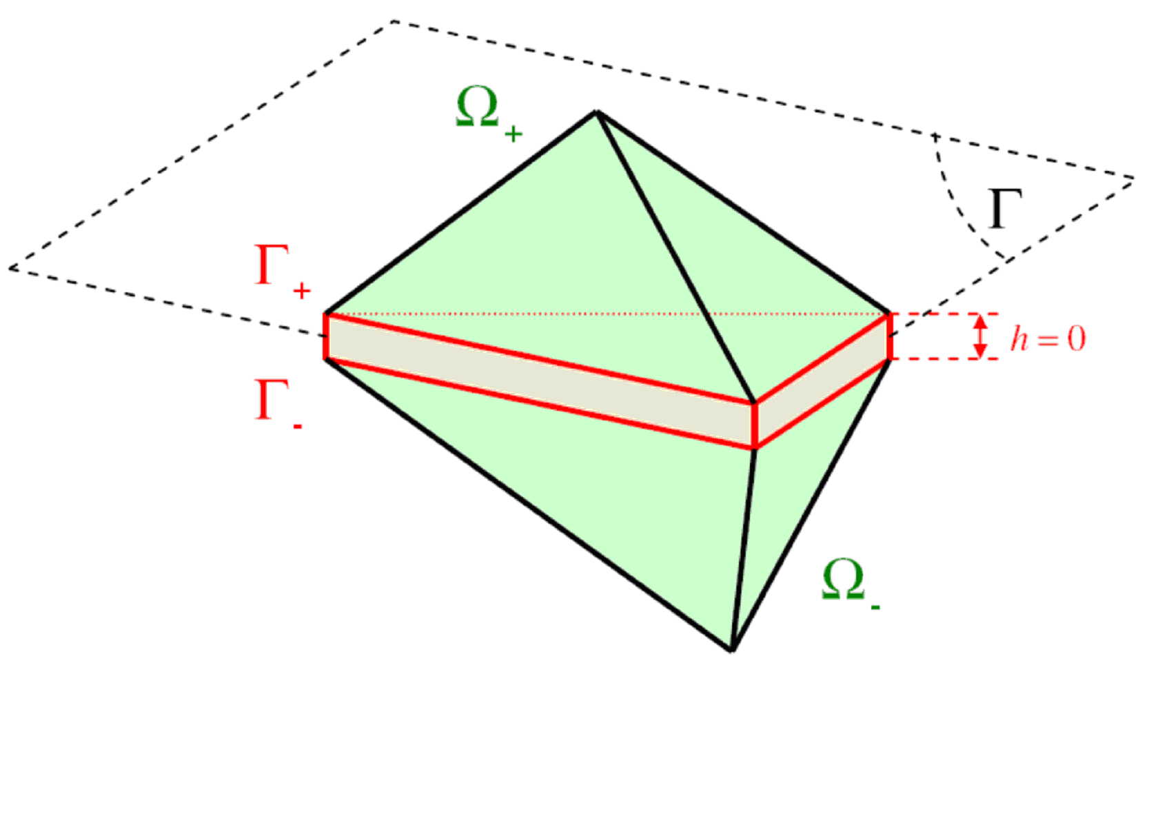
Figure 3.1-a: 3D diagram of an element \(\mathrm{EI}\) or \(\mathrm{EJ}\) inserted between two tetrahedra.
For the surface models (\(\mathrm{EJ}\) and \(\mathrm{EI}\)), in 2D the lips of the crack correspond to the long sides of the cohesive elements (degenerate quadrangles), in 3D the lips are defined by the triangular faces (for degenerate pentahedra) or rectangular faces (for degenerate hexahedra) faces. For the element with internal discontinuity \(\mathrm{ED}\), the crack passes through the center of the element and is parallel to the two opposite sides. The models \(\mathrm{EJ}\) and \(\mathrm{ED}\) have a linear interpolation of the displacements, they are compatible with a linear volume mesh \(\mathrm{Q1}\) or \(\mathrm{P1}\). \(\mathrm{EI}\) has a quadratic interpolation of the displacements and is compatible with \(\mathrm{Q2}\) or \(\mathrm{P2}\) quadratic volume cells.
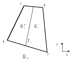
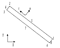
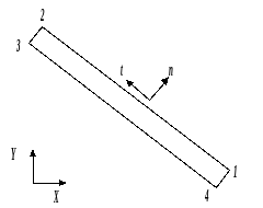
\(\mathrm{EI}\) \(\mathrm{EJ}\) \(\mathrm{ED}\)
Figure 3.1-b: 2D diagram of cohesive elements
3.2. Creating the mesh#
In this part, we give the tools available in Code_Aster to guarantee the good realization of a mesh with a cohesive crack and then we provide advice for the GMSH and Salomé landlords.
3.2.1. Code_Aster tools#
The meshes of the cohesive elements \(\mathrm{EI}\) and \(\mathrm{EJ}\) are surface, their orientation is defined by a local coordinate system, so it is necessary for their local connectivity to be defined a priori. This is also the case with \(\mathrm{ED}\), which are bulky since they are crossed by a surface discontinuity.
Two techniques are available in*Code_Aster* to perform this task. The first, once the mesh has been created, consists in verifying that they have a local numbering ad hoc (orientation). The second consists in meshing cohesive elements from two groups of opposing nodes (automatic creation).
Remarks :
The thickness of the elements \(\mathrm{EJ}\) and \(\mathrm{EI}\) has no influence on the solution. However, the latter can modify the dimensions of the structure; the user must mesh accordingly. When possible, it is recommended to make meshes of zero thickness.
For post-processing in 2D, a small thickness can however facilitate the visualization of variables at the gauss points (this problem does not occur in 3D because we are visualizing a surface) .
On the other hand, the \(\mathrm{ED}\) necessarily have a non-zero thickness. It is recommended to choose a size of the same order of magnitude as that of the surrounding non-cohesive elements.
Orientation
The keyword ORIE_FISSURE (command MODI_MAILLAGE) makes it possible to ensure the correct local numbering of the cells and to renumber correctly if necessary. For more details on how to use this procedure see [U4.23.04]. It is recommended to systematically use this command, which works in 2D and 3D (provided that the thickness of the cells is not zero) and regardless of the type of cohesive elements (linear or quadratic). An example of use for the cohesive layer “JOINT” is given:
MA= MODI_MAILLAGE (reuse =MA,
MAILLAGE =MA, ORIE_FISSURE ** =_F (GROUP_MA =” JOINT “),
Automatic creation
Another possibility: CREA_FISS allows the creation of cohesive meshes from two groups of nodes (facing each other or combined two by two). Some precautions are required when using this command, so it is advisable to read the documentation in CREA_MAILLAGE [U4.23.02]. This feature is available in 2D (the 3D equivalent is possible with a Salome python, see 12 below), here is an example from node groups GN1 and GN2.
MA = CREA_MAILLAGE (
MAILLAGE = MA_INI,
CREA_FISS = (
_F (NOM =” JOINT “, GROUP_NO_1 =” GN1”, =” “, GROUP_NO_2 =” GN2”, PREF_MAILLE =”MJ”),
))
Remarks:
Once order CREA_FISS has been made, it is not necessary to place the ORIE_FISSURE reel if you are creating a linear mesh.
If you want to use this procedure with the interface elements (therefore quadratic meshing), you must first perform the previous procedure on a linear mesh, then switch to quadratic ( LINE_QUAD/TOUT =” OUI “) and finally go over the pinette ORIE_FISSURE on the cohesive layer because the command LINE_QUAD a can be modified the local numeration.
Finally, tools are being developed to facilitate the creation of cohesive meshes. Especially in Salome version 5 (see 12).
3.2.2. Tips GMSH#
With free mesh GMSH, it is quite easy to build a layer of cohesive finite elements intended to be joint or interface elements regardless of the nature of the volume mesh. Just use the « Extrude » command and take a few precautions.
In 2D: we extrude a line n from one edge of the domain, with a thickness ep (small but not zero) in the -Y direction, and we specify that we only want a layer of elements with the keyword « Layers », finally we add « Recombine » so that the mesher creates quadrangles (triangles by default).
ep=0.001
Nblayer = 1;
JOINT [] =Extrude Line {n, {0, -ep,0}}
{
Layers {nbLayer,1}; Recombinge;
};
Then we can define a « Physical Line » of the new line created or a « Physical Surface » of the surface created in the following way:
Physical Line (a) = {JOINT [0]};
Physical Surface (b) = {JOINT [1]};
The first can be used for example to apply symmetry boundary conditions, the second corresponds to the layer of cohesive elements. If you want to include the crack inside a domain, you proceed as before, then you extrude the new line JOINT [0] to create the second part of the volume.
In 3D: we proceed in the same way with the extrusion of a border surface of the domain, the « Recombine » makes it possible to create hexahedra if the trace of the mesh on the extruded surface includes quadrangles and pentahedra if the latter includes triangles.
Finally, the « physical » ones created in the .geo file are used in the .comm command file in the usual way:
Physical Line (i) corresponds to “GMi” if the mesh is in .msh format
Physical Surface (j) corresponds to “GMj” if the mesh is in .msh format
Physical Line (k) corresponds to “G_1d_k” if the mesh is in .med format
Physical Volume (l) corresponds to “G_3d_l” if the mesh is in .med format
Attention :
There is a bug in GMSH 2.3 for 3D extrusion with the mesh algorithm “Tetgen+Delaunay”. This algorithm is the one proposed by default, so it is necessary to modify it in the Option/Mesh/General menu and choose 3D Algorithm=”NetGen”. This bug is listed on the GMSH website and should be changed in future releases.
Remarks :
The meshes created by GMSH are topologically correct but the local numbering of the nodes is not necessarily well done. In Code_Aster the latter must be defined in a specific way in order to distinguish the orientation of the cohesive elements. After reading the mesh in .msh or.med format it is therefore necessary to go through a MODI_MAILLAGE with the command ORIE_FISSURE which carries out this operation of renumbering the cohesive elements automatically (see part 10 ) .
Note that the extrusions mentioned above are also easily carried out interactively using the mouse. Once the.geo is automatically generated, however, you must add the « Recombin* » to create 2D quadrangles or 3D hexahedrs/pentahedra.*
3.2.3. Salome Tips#
In Salomé, it is possible to extrude a layer of surface elements from one edge of the domain. This makes it possible to create cohesive meshes whose connectivity can be changed if necessary using the ORIE_FISSURE command (see part 10).
- Work is in progress to mesh cohesive elements between two volumes or along a surface layer within a volume. The python doubleNodeGroups command [1] _
allows you to split the nodes of a group of surface elements or a given group of nodes (see module reference manual MESH). The weaving of cohesive elements between these two groups of nodes can then be done in 2D in the command file using the CREA_FISS keyword (see part 10) or from a python script [2] _
in 3D.
Note :
Regardless of the technique adopted to mesh the potential crack path, it is necessary for this one to cross both sides of the structure. Indeed, there are no cohesive finite elements intended to model a crack point (triangle for example) that cannot be propagated. Moreover, this would not really make sense since it is contrary to the logic of modeling a potential path.
3.2.4. Case of advanced geometric configurations#
When using finite interface elements (FEs), the presence of two families of degrees of freedom, displacements, and cohesive (augmented) forces complicates the management of advanced geometric configurations. This expression refers to situations in which several interfaces intersect, lead to one another, lead to a condition with kinematic boundaries or even present a border in the volume and not at one edge of the structure.
Advice on how to mesh such configurations was given in note [bib9]. It is observed that it is the knots that carry the degrees of freedom corresponding to the cohesive forces that require particular care.
3.3. Cohesive zone modeling#
A crack CZM is defined by three zones, the first corresponds to a crack free of stress, the second, called a cohesive zone, where the cohesion forces are non-zero and finally a healthy zone (or zone of potential cracking) where the priming stress has not been reached (see figure 3.3).
The cohesive zone allows for a gradual transition from healthy material to a real crack. The size of this last one is linked to the characteristic length \({G}_{c}/{\sigma }_{c}\) of the cohesive model, it adapts to remove the singularity of the stresses at the crack point. The shorter this length, the smaller the size of the cohesive zone will be. At the limit, if it tends to zero, the cohesive zone disappears and we find ourselves in the case of classical fracture mechanics with the theoretical possibility of having infinite stresses at the crack point. Formally, this is equivalent to taking an infinite \({\sigma }_{c}\) breaking constraint.
The importance of correctly simulating this cohesive zone is emphasized here, both from a mechanical and numerical point of view. In general, and regardless of the type of calculation, it is advisable to mesh this zone sufficiently so that it is composed of at least four or five cohesive finite elements. This makes it possible to finely represent the evolution of the crack on a mechanical level but also makes it possible to avoid numerical convergence problems associated with too rough discretization of this zone with a high stress gradient.
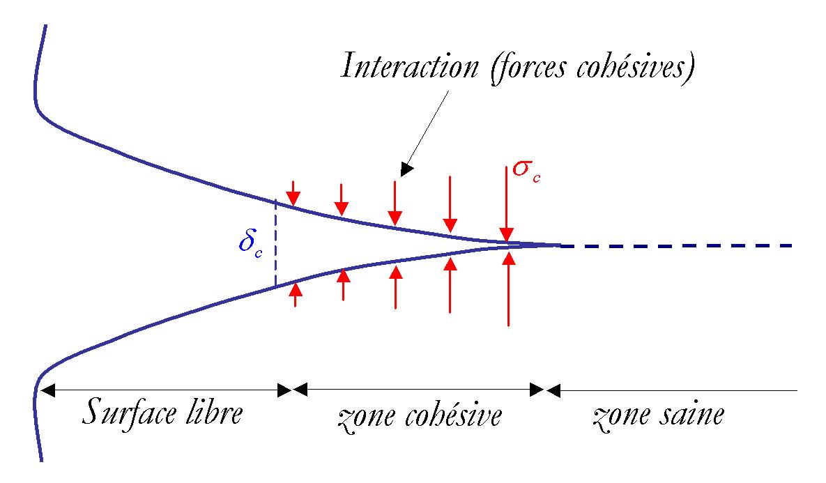
Figure 3.3: Diagram of the cohesive crack.
In the literature [bib7] there is an estimate of the size of the cohesive zone \({S}_{\mathrm{zc}}\) for a crack in an infinitely elastic material:
\({S}_{\mathrm{zc}}\simeq \frac{E}{1-{\nu }^{2}}\frac{{G}_{c}}{{\sigma }_{c}^{2}}\)
with \(E\) Young’s modulus, \(\nu\) Poisson’s ratio. This value is given as an indication to estimate the size of the cohesive zone, however the cohesive zone may vary with different parameters of the mechanical problem.
3.4. Definition of a cohesive pre-crack#
In most cases, cohesive elements are arranged in a crack plane or as an extension of an existing crack. The latter is generally represented by a free surface. However, in some cases, it may be useful to place cohesive meshes on an initial crack. The latter can for example be used as contact elements (small deformations) or used to define initial plane or semi-elliptical crack fronts for example.
To define an initial crack, it is necessary to build a mesh with two zones of contiguous cohesive elements, one for the pre-crack and the other for the potential crack. The idea then consists in imposing the internal variables of the pre-crack in such a way that they correspond to a zone free of stress, and not to modify those of the potential crack (i.e. setting them to 0). To do this, we use CREA_CHAMP commands to build an internal variable field at the gauss points. The latter is then used as the initial input state in STAT_NON_LINE with the ETAT_INIT command. Note that it is necessary to define all the internal variables of the structure, including those of the volume part. In the case of an elastic material, this operation is trivial, since it is non-linear, it is not possible to know them easily unless they are null and void, which is not necessarily realistic.
Note :
It is not possible to define an initial crack by imposing the material parameters \({\sigma }_{c}\) and \({G}_{c}\) null.
3.5. Multi-cracking#
It is possible to model several cracks with all types of cohesive elements as long as the meshing is done accordingly. With the ED element, for example, it is possible to arrange layers of elements in order to take into account a network of parallel cracks (see example [bib5]). For the EJ and EI elements, the holed plate test (ssnp133 [V6.03.133]) makes it possible to model the simultaneous advance of two cracks.
However, with this type of approach, it is not recommended to have cohesive elements everywhere (i.e. on each edge of the mesh). In addition to the difficulty in producing such a mesh, numerous works in the literature show that the results of the crack path are highly dependent on the mesh. Moreover, for EJs, the regularization of the cohesive law can also contribute to the variability of results and play a harmful role on the quality of the solution. Finally, this raises the non-trivial question of the conditions to be respected at the intersection of two cracks. No particular treatment is carried out for the models presented here.