8. Separation and fusion of crack fronts#
Different methods have been presented to follow the propagation of a crack with X- FEM (i.e. to update the values of the level-sets at each propagation step):
The mesh method (or by projection), see paragraph § 7,
The geometric method, see paragraph 6.
Upwind and simplex methods based on fast marching algorithms
The aim is to explain here the modifications to be made to these various methods to account for the behavior of a crack front when it encounters an obstacle (a hole for example). How to manage the separation of this crack front into two, or even several other pieces? Likewise, what about the fusion of two independent crack fronts into one? Level-sets determine the crack base and therefore the presence or absence of several crack bottoms. But in some cases, it is a question of making improvements to the previous methods so that they adapt to the separation of the crack front (modification of the creation of the crack mesh for the mesh method, continuity of the level-sets in the hole for the upwind method with the use of an auxiliary grid).
Depending on the methods used to manage the update of level-sets, the strategy put in place to account for the separation or fusion of crack fronts differs.
8.1. Meshing method#
For the mesh method, a first option is to extend what is done in paragraph 7.2 to the framework of several crack bottoms. Level-sets give information on the number and position of the ends of the crack bottoms (intersection between the structure’s mesh and the iso-zero of the two level-sets). While maintaining the nodes that constitute the endpoints that already exist at instant \(i-1\), the nodes constituting the new endpoints are selected (figure a.).
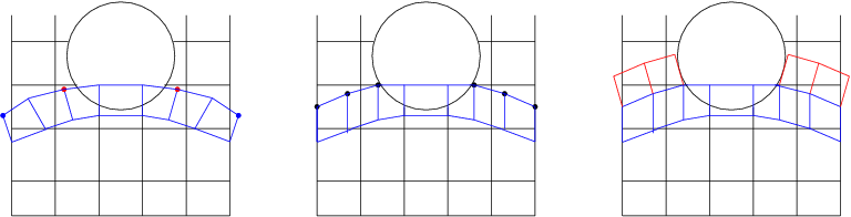
Figure 8.1-1 : a. nodes determining the ends of the crack bottoms (in blue: nodes selected for the already existing ends, in red: nodes selected for the new ends), b. repositioning the selected nodes on the different backgrounds, c. calculation of the propagated nodes and formation of new meshes.
As in paragraph 7.2, a procedure for repositioning the nodes of the various funds (figure b.) is carried out. All that remains is to calculate the propagated nodes and form the meshes (figure c.).
Although this method works correctly, it has one disadvantage: the loss of knots when two funds are separated. In addition, the meshes can be significantly deformed during the phase of repositioning the knots external to the structure. In particular, this can lead to poor discretization of the crack when propagating out of plane.
To overcome these difficulties, the idea was to increase the number of knots on each crack background. There is still the question of creating these nodes and meshing. By noticing that the cells representing the crack are only used to make projections, it is possible to create a row of cells for the advance of cracks that do not conform to the previous row of cells (figure). In this way, it is possible to increase the number of nodes between two propagation steps without modifying the discretization induced by the propagation speeds.
The algorithm is therefore summarized as follows: search for the nodes closest to the ends of the bottom, repositioning on the edge, creation of new nodes on the current background positioned equidistant from each other, calculation of the nodes of the new bottom. As there are the same number of nodes between the two backgrounds, quadrangles that respect the surfaces of the background are created.
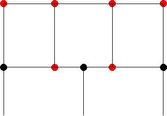
Figure 8.1-2 :: ** non-compliant mesh (in red; knots created for the new mesh row). The total number \(N\) of nodes on all crack bottoms must remain constant between two propagation steps. To do this, we distribute the \({N}_{i}\) knots per bottom in proportion to the ratio between the curvilinear length \({s}_{i}\) of the bottom \(i\) and the total curvilinear length of the \(n\) bottoms:
Where \(E(x)\) represents the integer part of \(x\). As there may be cases where the sum of \({N}_{i}\) is less than \(N\), the remaining nodes are distributed to the funds with the largest decimal part.
Note:
The mesh method can be problematic when the crack is concave. This case can in particular be encountered when two crack backgrounds are combined (figure a.) and is absolutely to be avoided because significant problems are created by the calculation of level-sets (false values, appearance of false crack backgrounds).
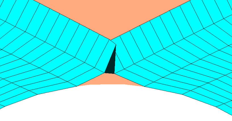

Figure 8.1-3 : problem cases: a.concave crack front when two crack bottoms meet, b. creation of pathological meshes.
The creation of problem meshes (concave for example) can prove to be a source of difficulties (see figure b.). It can occur when the propagation speed for the nodes on the edge is imposed tangent to the surface. It can also create errors in the tangent level-set calculation and involve the creation of false crack bottoms. To avoid the concavity of a mesh in the case of too great a maximum advance \({\mathit{Da}}_{\mathit{max}}\) of the crack, the value of the latter is reduced for the following calculation. Let the quadrangle represented in the plane \((\mathrm{ABC})\) figure (if the quadrangle is not plane then the point \(D\) represents the projection of the node propagated from \(C\) on the plane \((\mathrm{ABC})\)). We calculate the coordinates of the point \(M\) of intersection between \((\mathit{AB})\) and \((\mathit{CD})\) and we compare the distances between \(\mathit{AM}\) and \(\mathit{AB}\), \(\mathit{CM}\) and \(\mathit{CD}\). We put \(\left(\vec{{E}_{1}}=\frac{\vec{\mathit{AB}}}{∣∣\vec{\mathit{AB}}∣∣},\vec{{E}_{2}}=\frac{\vec{\mathit{AC}}-(\vec{\mathit{AC}}\mathrm{.}\vec{{E}_{1}})\vec{{E}_{1}}}{∣∣\vec{\mathit{AC}}-(\vec{\mathit{AC}}\mathrm{.}\vec{{E}_{1}})\vec{{E}_{1}}∣∣}\right)\) as an orthonormal base, and \(\vec{\mathit{AD}}({d}_{\mathrm{1,}}{d}_{2})\), \(\vec{\mathit{AC}}({c}_{\mathrm{1,}}{c}_{2})\), and \(\overrightarrow{\mathit{AM}}(x\mathrm{,0})\) in the \((A,\vec{{E}_{1}},\vec{{E}_{1}})\) frame, and,, and. By definition of \(M\), \(\mathit{det}(\vec{\mathit{CM}},\vec{\mathit{CD}})=∣\begin{array}{cc}x-{c}_{1}& {d}_{1}-{c}_{1}\\ -{c}_{2}& {d}_{2}-{c}_{2}\end{array}∣=0\).
We deduce \(x\mathrm{=}\frac{{d}_{2}{c}_{1}\mathrm{-}{d}_{1}{c}_{2}}{{d}_{2}\mathrm{-}{c}_{2}}\mathrm{=}\frac{(\overrightarrow{\mathit{AD}}\mathrm{.}\overrightarrow{{E}_{2}})(\overrightarrow{\mathit{AC}}\mathrm{.}\overrightarrow{{E}_{1}})\mathrm{-}(\overrightarrow{\mathit{AD}}\mathrm{.}\overrightarrow{{E}_{1}})(\overrightarrow{\mathit{AC}}\mathrm{.}\overrightarrow{{E}_{2}})}{\overrightarrow{\mathit{CD}}\mathrm{.}\overrightarrow{{E}_{2}}}\).
The coefficient \(\mathit{Crit}=\mathit{min}\left(\frac{\mathit{AM}}{\mathit{AB}},\frac{\mathit{CM}}{\mathit{CD}}\right)\) is introduced and the rectified maximum progress \({\mathit{Da}}_{\mathit{max}}\text{'}\) verifies:
\(\mathit{si}\phantom{\rule{4em}{0ex}}\mathit{Crit}\phantom{\rule{0.5em}{0ex}}<\phantom{\rule{0.5em}{0ex}}1.2\phantom{\rule{10em}{0ex}}\mathit{alors}\phantom{\rule{4em}{0ex}}{\mathit{Da}}_{\mathit{max}}\text{'}\phantom{\rule{0.5em}{0ex}}=\phantom{\rule{0.5em}{0ex}}\frac{{\mathit{Da}}_{\mathit{max}}\mathrm{.}\mathit{Crit}}{1.2}\)
Figure 8.1-4 : representation of a mesh for which we check that the progress is not too great. The coefficient \(\mathrm{1,2}\) is a safety coefficient in order to ensure non-zero propagation (\(\mathit{Crit}=1\) leading to a point \(M\) coinciding with the point (s) \(B\) and/or \(D\)).
Although with such a strategy, maximum progress is likely to tend towards 0, it does however make it possible to solve some of the problem cases.
8.2. Upwind method: introduction of a virtual background#
As noted in paragraph 4.2.1.4, the use of the upwind method is very generally accompanied by the use of an auxiliary grid (whose mesh is regular) on which the level-sets are updated, which are then projected onto the physical mesh of the room (generally much less regular). However, part of the grid may be located outside the mesh of the part, as for example in the case of a structure containing a hole.
The grid nodes located outside the room’s mesh are then projected onto the same point on the crack front when calculating the propagation speed of the level-sets. All these nodes are therefore assigned the same speeds and angles of propagation as well as the same local bases (as described in paragraph 2.3). This results in the appearance of a discontinuity of the level-sets on the grid at the free edge of the piece (see figure).
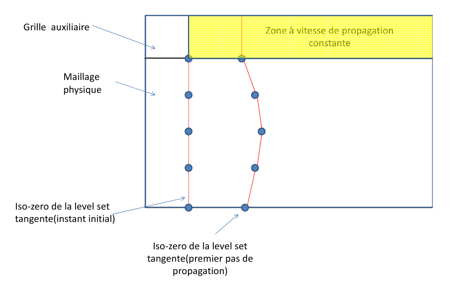
Figure 8.2-1 : example of discontinuity of level-sets on the grid at the free edge. This discontinuity, although located outside the physical mesh, implies a poor definition of the level-set gradient on the free edge and therefore a poor definition of the local base during the next propagation step. It can also influence the definition of level-sets within the mesh, in particular during the propagation of cracks in parts with irregular sections and/or holes. To avoid these problems and to define consistently the level-sets on the grid in the vicinity of the physical mesh, an interpolation of the crack front outside the mesh by a line tangent to the crack front is proposed. To do this, the last segment of the crack front is extended by a straight segment at the end of which a new crack front node, qualified as virtual, is introduced. This point is then considered to be a point on the crack front. It is assigned the same local base as that of the last point of the physical crack front. The speed and the angle of propagation are calculated by linear interpolation from the speeds and angles of propagation of the last two points (figure).
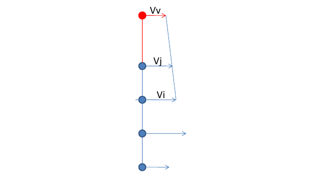
Figure 8.2-2 : representation of the linear approximation of the speed at the virtual point \({V}_{v}\) (in red) from the speeds of the last two points on the crack front \({V}_{i}\) and \({V}_{j}\) (in blue) .
To create the points of the virtual background, proceed as follows (figure):
we place \({P}_{i}\) and \({P}_{j}\) two points located at the end of the crack font and \(d\) the distance from the virtual point \({P}_{v}\) to the last point at the bottom of the crack \({P}_{j}\),
we determine the line extending the last segment of the crack front to the virtual point: \(\overrightarrow{{P}_{\mathit{jv}}}\mathrm{=}\mathit{d.}\overrightarrow{{b}_{j}}\) where \(\overrightarrow{{P}_{\mathit{jv}}}\) is the vector connecting \({P}_{j}\) to \({P}_{v}\) and \(\overrightarrow{{b}_{j}}\) is the unit vector tangent to the crack front at the point \({P}_{j}\),
we calculate the spatial derivatives of the speed and the angle of propagation on the last segment of the virtual background:
we deduce the speed and the angle of propagation at the virtual background:
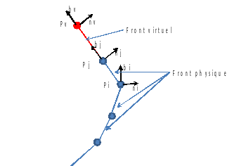
Figure 8.2-3 :creation and location of the virtual crack front. The virtual point is placed at a distance \(d\) from the physical front equal to the radius of the torus used for the propagation of the level-sets (see paragraph 5). This distance is chosen so as to obtain level-sets that are smoothed over the entire propagation zone. If the location is not used, the virtual point is placed at a distance of seven times the maximum advancement of the crack. For speeds and angles of propagation (defined on the virtual points) that are too large or too low, the virtual point is brought closer to the physical front so as to satisfy the conditions imposed. For example, we note that there is a significant discontinuity in level-sets if the angle of propagation is greater than (respectively less) than 90 degrees (respectively -90 degrees). It should also be noted that if the distance from the virtual point to the physical crack front is less than the radius of location, it is possible to maintain a discontinuity of the gradients. However, this discontinuity is located far from the mesh of the part. It therefore does not affect the definition of the local base on the free edge.
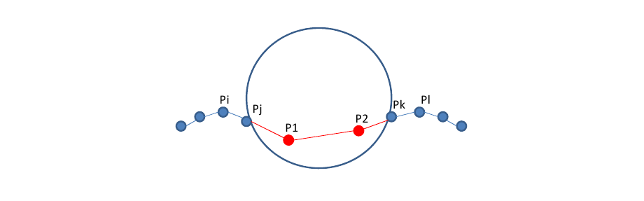
Figure 8.2-4 : creating a virtual front (in red) inside a circular hole. \({P}_{1}\) is created by extending of \([{P}_{i}{P}_{j}]\) and \({P}_{2}\) by extending of \([{P}_{l}{P}_{k}]\) *. The last segment of the virtual background connects*\({P}_{1}`** and**:math:`{P}_{2}`** and connects the crack fronts. ** The virtual background method can then be immediately extended to the case of holes. If the room has a hole, it is also important to clearly define the level-sets inside this one. We then proceed as described above by defining a virtual crack front inside the hole by creating two virtual points :math:`{P}_{1}\) and \({P}_{2}\), one for each crack background delimited by the hole (figure). Two of the three segments of the virtual front are extensions of the two physical crack fronts. The third segment connects the two virtual points in order to connect the crack fronts. It is not used to interpolate the level-sets but to ensure their continuity in the hole. Since the two virtual points have different propagation speeds, two neighboring nodes located in the center of the hole can be projected onto two different crack bottom nodes and have different speeds.
The propagation angles and speeds as well as the local base on segment \([{P}_{1}{P}_{2}]\) are calculated by linear interpolation (as described in paragraph 2.4) from the values assigned to the two virtual points.
In the case of creating a virtual background in a hole, it must be ensured that there is no crossing of the crack bottoms. The distance from a virtual point to the bottom of the crack must not exceed one third of the distance between the two bottoms. Either:
In addition, the propagation speed at virtual point \({V}_{v}\) should not be too small or too large. It is required that it be at least equal to two thirds of the speed Vj of the last crack bottom and that it must not exceed four thirds of this value. Thus, it is required that:
Likewise:
: label: eq-71
textrm {Yes} {V} _ {v} <frac {2 {V} _ {j}} {3}
And:
We deduce the expression for distance \(d\) in these two cases:
However, creating a virtual fund is not enough. The values of the level-sets defined inside the hole, resulting from the projection onto the middle segment of the virtual background, can in some cases influence the definition of the level-sets in the mesh. In addition, the speed approximation is more accurate if the level-sets are initially straight and if the intersection of the two iso-zeros is confused with the virtual front. In order to guarantee the straightening of the level-sets in the hole during the fusion of the crack fronts after the passage of this one, the level-sets are recalculated for the nodes projected onto a virtual segment of the crack front, and this before the level-sets propagate. Level-sets are calculated geometrically (see paragraph 6) by projecting the node onto the crack front (figure). We place \(\mathit{XM}\) a mesh node. Its projection \(\mathit{XN}\) is then defined on the crack background, the vectors \(\vec{\mathit{tp}}\) and \(\vec{\mathit{np}}\) defining the local base at the crack front in \(\mathit{XN}\). We get the normal and tangent level-sets at nodes \(\mathit{XM}\) simply by: \(\mathit{lsn}(\mathit{XM})\mathrm{=}\overrightarrow{\mathit{XM}\mathit{XN}}\mathrm{.}\overrightarrow{\mathit{np}}\) and \(\mathit{lst}(\mathit{XM})\mathrm{=}\overrightarrow{\mathit{XM}\mathit{XN}}\mathrm{.}\overrightarrow{\mathit{tp}}\).
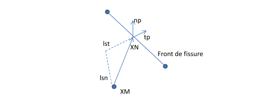
Figure 8.2-5 : Calculation of level-sets at the nodes projected onto the crack background. This calculation of the level-sets makes it possible to correct the influence of the non-physical definition of the level-sets at the center of the hole during the fusion of the two crack bottoms. Once the virtual background has been created and the level-sets have been corrected, the calculation of the propagation velocities by projection onto the crack front is performed as described in paragraph 2.3, without distinguishing between the physical front and the virtual background.
Note:
The introduction of a virtual background requires a strategy for verifying the numbering of the crack fronts as well as their direction of travel, which was previously not necessary: the connection of the crack fronts by a virtual background no longer makes them independent of each other. The following method has been adopted to check whether the nodes of the various crack fronts are correctly numbered (figure):
a new crack front is constructed on the auxiliary grid which, by definition of the grid, consists of only one piece with a single direction of travel. The ends \({E}_{1}^{i}\) and \({E}_{2}^{i}\) of each of the pieces \(i\) of the real crack front are then projected onto the continuous crack front associated with the grid. These ends are identified on the crack front of the grid by their respective curvilinear abscissa. For example, the curvilinear abscissa \({s}_{{P}_{1}^{i}}\) and \({s}_{{P}_{2}^{i}}\) correspond to the ends \({E}_{1}^{i}\) and \({E}_{2}^{i}\) (where \({P}_{1}^{i}\) and \({P}_{2}^{i}\) are respectively the projections of \({E}_{1}^{i}\) and \({E}_{2}^{i}\) onto the crack front associated with the auxiliary grid);
the sequence of curvilinear abscissa thus obtained allows renumbering the pieces of the fronts of the real crack;
we evaluate the dot product \(({E}_{2}^{i}{E}_{1}^{i})\mathrm{.}({P}_{2}^{i}{P}_{1}^{i})\) to verify that each of the pieces is traveled in the same direction as the crack front on the grid. Otherwise, the misoriented piece (s) is reoriented.
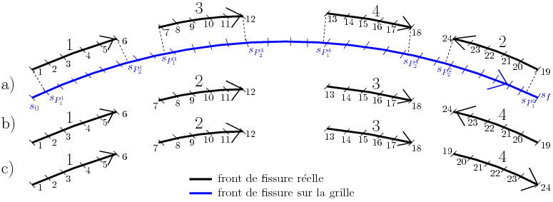
Figure 8.2-6 : a. example of incorrect numbering and orientation of the real crack front (black) and crack front on the grid (blue), b. renumbering the pieces of the real crack front, c. reorientation of the pieces of the real crack front
8.3. Geometric and simplex method#
Since the geometric method and the simplex method do not require any auxiliary grid, the management of the separation and fusion of crack fronts is automatic and does not require any particular modification.