2. Calculation of the propagation speed field#
The first steps consist in calculating two speed fields, normal and tangential, defining the dissociated evolution of the two level-sets. We are placing ourselves in the context of a mixed mode of propagation.
2.1. Rate of advance of the bottom of the crack#
The advance of the bottom of the crack at each of its points evolves in the local base according to a Paris law. Its direction can be determined by several criteria detailed in paragraph [§ 2.7]. You can generally write:
Or again:
And where \(C\) and \(m\) are characteristics of the fatigue behavior of the material, \(G\) is the local energy restoration rate from the \(G\) -Theta method, and \(\mathrm{\beta }\) is the connection angle. This angle is equal to:
Or even:
: label: eq-4
mathrm {beta} =2mathrm {arctan}left [frac {1} {4}mathrm {.} left (frac {1+ {x} _ {I} - {I} - {(1- {x}} _ {mathit {III}})} ^ {p}} {text {} {x} _ {mathit {II}} _ {mathit {II}} _ {mathit {x}} _ {mathit {II}} _ {mathit {x}} _ {mathit {x} _ {mathit {x}} _ {mathit {x} _ {mathit {II}} _ {mathit {x} _ {mathit {II}} _ {mathit {II}} _ {mathit {II}} _ {mathit { sqrt {{(frac {1+ {x} _ {I} _ {I} - {(1- {x}} _ {mathit {III}})} ^ {p}} {text {} {x}} _ {mathit {x}} _ {mathit {II}}}} - {(1- {x}} _ {mathit {II}}}})} ^ {p}}} {text {} {x}} {text {} {x} _ {x} _ {mathit {II}}}})} ^ {2} +8}} {text {} {
With:
:math:`{x}_{i}=frac{{K}_{i}}{{K}_{I}+left |
{K}_{mathit{II}}right |
+left |
{K}_{mathit{III}}right |
}` and \(p=\frac{\sqrt{\mathrm{\pi }}-5\mathrm{\nu }}{4}\) |
2.2. Velocity field extended to the mesh#
The normal and tangent velocities are known only for the points of intersection between the bottom of the crack and the faces of the mesh elements. These points are not nodes in the mesh. To update level-sets after a propagation, the speed must be known for each node in the mesh [§ 3.1]. It is therefore necessary to extend the speed to all the nodes of the mesh based on the values on the crack background. To do this, each node is projected onto the crack bottom in the normal direction and the node is assigned the speed of the point, which is the projection of the node.
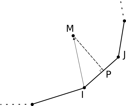
Figure 2.2-1 : projection of the knot \(M\) on the background of a crack The projection is implemented according to the following algorithm ():
Loop on the \(\text{M}\) nodes of the mesh
Initialization: \({d}_{\mathit{min}}\mathrm{=}\text{réel maxi}\)
Loop on segments \(\overrightarrow{\text{IJ}}\): between two consecutive points \(I\) and \(J\) at the bottom of the crack
We calculate \(s=\frac{\vec{\text{IJ}}\cdot \vec{\text{IM}}}{{\Vert \vec{\text{IJ}}\Vert }^{2}}=\frac{\Vert \vec{\text{IP}}\Vert \cdot \Vert \vec{\text{IJ}}\Vert }{{\Vert \vec{\text{IJ}}\Vert }^{2}}=\frac{\Vert \vec{\text{IP}}\Vert }{\Vert \vec{\text{IJ}}\Vert }\)
If \(s<0\), then \(s\mathrm{=}0\)
If \(s>1\), then \(s\mathrm{=}1\)
If you project node \(M\) onto \(\overrightarrow{\text{IJ}}\), you get point \(P\). The position of this point is determined by the vector \(\overrightarrow{\text{IP}}\): \(\overrightarrow{\text{IP}}\mathrm{=}s\mathrm{\cdot }\overrightarrow{\text{IJ}}\)
We calculate the distance between node \(M\) and its projection \(P\): \(d\mathrm{=}∥\overrightarrow{\text{MP}}∥\)
If \(d<{d}_{\mathit{min}}\), then we store \({d}_{\mathit{min}}\), \({\text{I}}_{\mathit{min}}\mathrm{=}\text{I}\),, \({\text{J}}_{\mathit{min}}\mathrm{=}\text{J}\), and \({s}_{\mathit{min}}\mathrm{=}s\)
End buckle
End buckle
The parameter \({s}_{\mathit{min}}\) gives the position of the projection \(P\) of each node \(M\) of the mesh in relation to the length of the vector \(\overrightarrow{{\text{I}}_{\mathit{min}}{\text{J}}_{\mathit{min}}}\) of the crack background to which the projection \(P\) belongs. The position of the projection \(P\) can therefore be considered as a parametric position on the vector \(\overrightarrow{{\text{I}}_{\mathit{min}}{\text{J}}_{\mathit{min}}}\). This can be used to calculate the value of the speed vector \(V\) to be assigned to node \(M\).
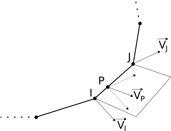
Figure 2.2-2 : determining the speed of the point \(N\) This problem is reduced to the determination of the speed vector \({V}_{P}\) of a point \(P\) of the segment \(\overline{\text{IJ}}\) when the speed vectors are known at the points \(I\) and \(J\) ().
The method used to calculate \({V}_{P}\) is arbitrary. If we look at the physical meaning of speed, we can say that it changes gradually between the two limit vectors \({V}_{I}\) and \({V}_{J}\) with the position of point \(P\). For the value of \(\Vert {V}_{P}\Vert\) we can therefore use a linear interpolation between the two values \(∥{V}_{\text{I}}∥\) and \(∥{V}_{\text{J}}∥\):
For the direction of \({V}_{\text{P}}\), we can determine the angle between \({V}_{\text{I}}\) and \({V}_{\text{J}}\) and once again use linear interpolation on the calculated angle, according to the following algorithm:
we calculate the vector normal to the plane formed by the vectors \({V}_{\text{I}}\) and \({V}_{\text{J}}\): \({v}_{3}\mathrm{=}{V}_{\text{I}}\mathrm{\wedge }{V}_{\text{J}}\)
we go back to a local base formed by the vectors \({V}_{\text{I}}\) and \({v}_{3}\). We calculate the last axis of the base: \({v}_{2}\mathrm{=}{v}_{3}\mathrm{\wedge }{V}_{\text{I}}\). This vector is in the plane formed by vectors \({V}_{\text{I}}\) and \({V}_{\text{J}}\).
we calculate the unit vectors of the base in this plane: \({u}_{1}=\frac{{V}_{\text{I}}}{\Vert {V}_{\text{I}}\Vert }\) and \({u}_{2}=\frac{{v}_{2}}{\Vert {v}_{2}\Vert }\)
we calculate the angle between the two speed vectors \({V}_{\text{I}}\) and \({V}_{\text{J}}\): \(\mathrm{\alpha }=\mathit{acos}\left(\frac{\sum _{i=1}^{3}{V}_{\text{I}i}\cdot {V}_{\text{J}i}}{\Vert {V}_{\text{I}}\Vert \cdot \Vert {V}_{\text{J}}\Vert }\right)\)
we calculate the unit vector of the speed at point \(P\) by linear interpolation:
\({u}_{\text{P}}\mathrm{=}\mathrm{cos}(\alpha {s}_{\mathit{min}})\mathrm{\cdot }{u}_{1}+\mathrm{sin}(\alpha {s}_{\mathit{min}})\mathrm{\cdot }{u}_{2}\)
finally we calculate the speed vector at point \(P\) using the value \(∥{V}_{\text{P}}∥\) already calculated: \({V}_{\text{P}}\mathrm{=}∥{V}_{\text{P}}∥\mathrm{\cdot }{u}_{\text{P}}\)
2.3. Calculating the speeds for each node in the mesh#
To make the normal level-set evolve appropriately [§ 2.5] and to integrate the two level-set updating equations [§ 3], we must know the normal speed vectors \({V}_{N}\) and tangent \({V}_{T}\) for each node in the mesh. To do this, simply calculate the normal and tangent directions of the level-sets using the gradients of the level-sets.
Unfortunately this solution is not applicable to all nodes. Indeed, after the update, the orthogonality property of the level-sets is not guaranteed [§ 4.1] for all nodes. This property is very important to ensure the orthogonality of the speed vectors \({V}_{N}\) and \({V}_{T}\). We must therefore use another solution.
Looking at the way used to extend the speed field to the nodes of the mesh [§ 2.2, § 2.5], we consider the following solution:
if the level-set tangent to the node is negative: it evolves in a direction parallel to the surface of the crack. We therefore use the gradients of the level-sets to calculate the normal and tangent directions. In effect, this means that the node is in the space of the existing crack and that the value of the normal level-set does not change during the update of the level-sets unlike the value of the tangent level-set [§ 2.5].
if the level-set tangent to the node is positive, the local base of the projection of the node on the crack background is used. Indeed, the evolution of the level-sets must be consistent with the modifications of the crack base.
For the first case, the calculation of the normal and tangent directions is not a problem because the gradients of the \(\mathrm{\varphi }\) level-sets at the nodes are always known: \({V}_{N}={V}_{N}^{\text{P}}\cdot \nabla {\mathrm{\varphi }}_{n}\) and \({V}_{T}={V}_{T}^{\text{P}}\cdot \nabla {\mathrm{\varphi }}_{t}\). However, the normal \({V}_{N}^{\text{P}}\) and tangent \({V}_{T}^{\text{P}}\) components of the speed \({V}_{\text{P}}\) must be calculated with respect to the local base of the crack bottom at point \(P\) using the following solution described for the second case.
In this case, the calculation is more difficult because the local base of the crack bottom is known only for the points of intersection between the crack bottom and the faces of the mesh elements. The situation is visible in figure: we know the local base at points \(I\) and \(J\) and we want to calculate the local base at point \(P\), projection of a node on the bottom of the crack. The orientation of this base must be between the orientations of the base at point \(I\) and of the base at point \(J\) according to the position of the point \(P\). The latter is well described by the parameter \({s}_{\mathit{min}}\) already calculated [§ 2.2].
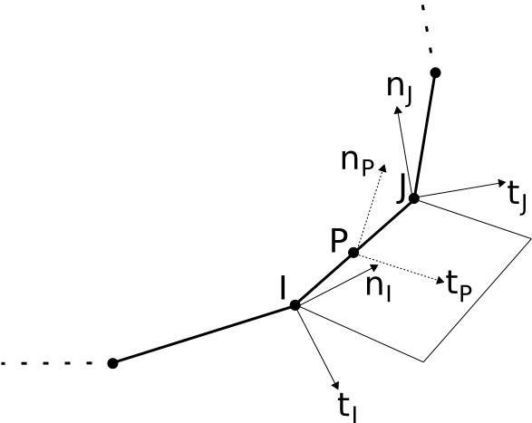
Figure 2.3-1 : determination of the local base at point \(P\)
If we do not consider the translation of the origin, the change in orientation of the local base can be seen as a rotation of the base from the orientation at point \(I\), for which \({s}_{\mathit{min}}\mathrm{=}0\). We have the maximum rotation for \({s}_{\mathit{min}}\mathrm{=}1\), that is to say at point \(J\). The orientation of the base at point \(P\) is obtained by using a lower rotation that is proportional to the value of \({s}_{\mathit{min}}\).
Using Euler’s theorem, one can always describe any rotation as a single rotation (Euler angle) around a single axis (Euler axis). The direction of the latter and the value of the rotation change for segment \(\overline{\text{IJ}}\) along the crack bottom.
The local base at point \(P\) can therefore be obtained by rotating around the Euler axis calculated for the rotation that transforms the base at point \(I\) into the base at point \(J\). The value of the angle of rotation can be calculated simply by multiplying the Euler angle by \({s}_{\mathit{min}}\). In the next paragraph [§ 2.4], we describe the equations we use for this calculation.
After determining the local base \({t}_{\text{P}}\) and \({n}_{\text{P}}\) at point \(P\), we can calculate the value of the components of the speed \({V}_{\text{P}}\). Either:
Finally, we calculate the two vectors \({V}_{N}\) and \({V}_{T}\):
In summary, for each node \(M\) of the mesh, the projection \(P\) on the crack background is calculated. Then we calculate the local base \({t}_{\text{P}}\) and \({n}_{\text{P}}\) at point \(P\) and the speed components \({V}_{\text{P}}\) (which have already been calculated [§ 2.2]):
Finally, we calculate the vectors \({V}_{N}\) and \({V}_{T}\) at the node \(M\) according to the sign of the tangent level-set:
Where \({\varphi }_{n}\) and \({\varphi }_{t}\) are the normal level-set and the tangent level-set respectively.
2.4. Calculating the local base#
As already described in the previous paragraph, we know the local base at points \(I\) and \(J\) and we want to calculate the local base at point \(P\) using a rotation.
The first step is to calculate the Euler axis and angle, which describe the rotation that must be applied to the base \(({t}_{I},{n}_{I},{b}_{I})\) at the point \(I\) to obtain the base \(({t}_{J},{n}_{J},{b}_{J})\) at the point \(J\). The algorithm used is as follows:
We calculate the third \(b\) axis of the local base at points \(I\) and \(J\). In fact, only the unit vectors \(t\) and \(n\) are stored:
We calculate the Euler rotation matrix between the two bases:
Each column in the matrix represents a vector from base to point \(J\) \(({t}_{J},{n}_{J},{b}_{J})\) in the local base to point \(I\).
We calculate the Euler angle using the elements of matrix \(\underline{\underline{{R}_{E}}}\):
We calculate the Euler axis \(e\mathrm{=}{\left[{e}_{1}{e}_{2}{e}_{3}\right]}^{\text{T}}\):
The calculated Euler angle and axis are the same for all points \(P\) on the edge defined by points \(I\) and \(J\). The second step is the calculation of the local base for a point \(P\) for which the position is determined by the parameter \({s}_{\mathit{min}}\) [§ 2.2]. The algorithm used is as follows:
We calculate the effective angle of rotation to use:
We calculate the rotation matrix between the local base at point \(I\) and the local base at point and the local base at point \(J\) for a rotation around the Euler axis \(e\) equal to \({\vartheta }_{P}\):
where matrix \(\underline{\underline{\epsilon }}\) is as follows:
We calculate the axes \({t}_{\text{P}}\) and \({n}_{\text{P}}\) from the local base at point \(P\) in the local base at point \(I\):
The two vectors are therefore coincident with the first and the second columns of the matrix \(\underline{\underline{{T}_{P}}}\). Using the above equation to calculate this matrix, we can therefore write:
And:
: label: eq-20
{n} _ {text {P} ({t} _ {I}, {n}}, {n} _ {I}, {b} _ {I})}mathrm {=}left [begin {array} {c} (1mathrm {-}mathrm {-}mathrm {-}}mathrm {-}}mathrm {cos} ({vartheta} _ {I})mathrm {P}}))mathrm {cdot} {e} _ {1}mathrm {cdot} {e} {e} _ {2} +mathrm {sin} ({vartheta} _ {text {P}})mathrm {cdot} {e} {e} {e} {e} _ {3} _ {3}\ mathrm {cos} ({vartheta}} _ {text {P}})mathrm {P}}) + (1mathrm {P}}) + (1mathrm {P}}) + (1mathrm {P}}) + (1mathrm {P}}) m {-}mathrm {cos} ({vartheta} ({vartheta}} _ {vartheta}}))mathrm {cdot} {e} _ {2}\ (1mathrm {-} -}mathrm {-}}mathrm {-}}mathrm {-}}mathrm {-}}mathrm {-}}mathrm {-}}mathrm {-}}mathrm {-}}mathrm {-}mathrm {-}}mathrm {-}}mathrm {-}}mathrm {-}}mathrm {-}}mathrm {-}}mathrm {-} _ {2}mathrm {cdot} {e} {e} _ {3}mathrm {-}mathrm {sin} ({vartheta} _ {text {P}})mathrm {cdot} {e} {e} {e} _ {1}end {array}right]
Finally, we can express the vectors \({t}_{\text{P}}^{\text{I}}\) and \({n}_{\text{P}}^{\text{I}}\) in the global mesh base, which is used for all calculations. If we denote the \(i\) component of the \({t}_{\text{P}({t}_{I},{n}_{I},{b}_{I})}\) vector by \({t}_{\text{P}({t}_{I},{n}_{I},{b}_{I})}(i)\) and the same component of the vector \({n}_{\text{P}({t}_{I},{n}_{I},{b}_{I})}\) by \({n}_{\text{P}({t}_{I},{n}_{I},{b}_{I})}(i)\), we can write:
: label: eq-21
mathrm {{}begin {array} {c} {c} {t} _ {text {P}}}mathrm {=} {t} _ ({t} _ {I}, {I}, {n}}, {n} _ {I}, {n} _ {I}, {n} _ {I}, {n} _ {I}, {n} _ {I}, {n} _ {I}, {n} _ {I}, {n} _ {I}, {n} _ {I}, {n} _ {I}, {n} _ {I}, {n} _ {I}, {n} _ {I}, {n} _ {I}, {n} _ {I}, {n} _ {I}, {n} t} _ {text {P} ({t} _ {I}, {n} _ {I}, {n} _ {I})} (2)mathrm {cdot} {n} _ {text {I}} _ {text {I}}}} + {text {I}}} + {t}} _ {I}} + {t}} _ {I}} (3)mathrm {cdot} {b} _ {text {I}} _ {text {P}}\ mathrm {=} {n} _ {text {P} ({t} {P} ({t} _ {I}, {I}}, {n}}, {n} _ {I}})} (1)mathrm {cdot} {P} (1)mathrm {cdot} {P} ({P}) (1)mathrm {cdot} {P} ({P}} (1)mathrm {P} {P}} (1)mathrm {P} {P}} (1)mathrm {P} {P} {b}} {n} _ {text {I}} + {n} _ {text {P} ({t}} _ {I}, {n} _ {I}, {b} _ {I})} (2)mathrm {cdot} {n} {n}} _ {n} _ {n} _ {I} _ {I} _ {I}, {n} _ {I} _ {I}, {n} _ {I}, {b} _ {I})} (3)mathrm {cdot} {b} _ {text {I}}end {array}
2.5. Adjusting the normal speed field#
In order to prevent the displacement of the pre-existing crack, and to make the normal level-set evolve appropriately, it is necessary to adjust the normal speed field (bib 1). We want to have a relatively smooth crack trajectory, such as:
The value of \(\Delta t\) is equal to the total integration time of the level-set update equations [§ 3.1]. Thus, the crack background is progressing well according to \({V}_{T}\) and \({V}_{N}\) calculated previously. We’re doing a linear approximation in \(\mathit{lst}\).
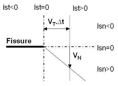
Figure 2.5-1 : Normal speed adjustment
The formula applied to all the nodes in the mesh is as follows:
Where \({V}_{N}\) and \({V}_{T}\) are the nodal velocity fields, and \(\Delta t\) the chosen time step (see paragraph [§ 3]).
2.6. Consideration of the spill#
In the case of a three-dimensional crack, two rotations are possible during the propagation of a crack. Consider a point at the bottom of crack \((P)\) with a local base associated with it (t, n, b). [bib 21] thus describes the rotation of plugging as the rotation of the speed vector \(V\) in the plane \((P,t,n)\) and \(\beta\) its associated angle, and the rotation of spill as being the rotation of the local base around the speed vector, of angle \(\mathrm{\gamma }\).
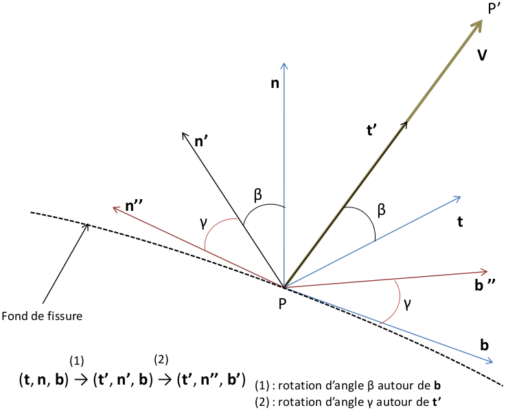
Figure 2.6-1: Definition of branch and discharge angles
Taking the spill into account therefore consists in rotating the local databases before the stage of updating the level-sets. The propagation stage therefore follows the following sequence:
application of plugging (\(\beta\)) and spill (\(\gamma\)) rotations to the local bases of the crack bottom points,
projection of the points of the mesh on the crack background,
allocation of a local base and a propagation speed \(V\) to all the projected points by interpolation between the points at the bottom of the crack,
update level-sets in local databases with speed \(V\).
Since the local databases were rotated before the level-sets were updated, the speed vector \(V\) is therefore carried only by the \(t\text{'}\) vector of the new local database. There is therefore no longer a normal speed component in the new local base.
Note:
Spill rotation can only be activated in 3D and when the key word CRIT_ANGL_BIFURCATION of the propagation operator PROPA_FISS is equal to SITT_MAX_DEVER.
By default the dump rotation is forced to \(0\) .
2.7. Determination of bifurcation angles#
In the case where the overflow is not taken into account, the branch angle is conventionally determined by the principle of the « Maximum Hoop Stress Criterion » [bib 4] according to the stress intensity coefficients \({K}_{I}\) and \({K}_{\mathit{II}}\) :
Note:
The branch angle can be calculated by the operator CALC_G [R7.02.05] [U4.82.03]. In this case it is imposed to PROPA_FISS in the same table as G and SIF.
It can also be calculated by the operator POST_RUPTURE [:external:ref:`U4.82.04 <U4.82.04>`] inside the operator PROPA_FISS [:external:ref:`U4.82.11 <U4.82.11>`]. This option allows you to choose other criteria*as the « Maximum Hoop Stress criterion ».
If the spill is taken into account, the branch angle and the spill angle are both calculated with the « Maximum Hoop Stress Criterion » [bib 21] using \({K}_{I}\), \({K}_{\mathit{II}}\) and \({K}_{\mathit{III}}\):
And for the angle of discharge:
With:
:math:`{x}_{i}=frac{{K}_{i}}{{K}_{I}+left |
{K}_{mathit{II}}right |
+left |
{K}_{mathit{III}}right |
}` and \(p=\frac{\sqrt{\mathrm{\pi }}-5\mathrm{\nu }}{4}\) |
Note:
The angle of spill is calculated by the operator POST_RUPTURE [:external:ref:`U4.82.04 <U4.82.04>`] inside the PROPA_FISS [:external:ref:`U4.82.11 <U4.82.11>`] operator when the latter’s CRIT_ANGL_BIFURCATION * **keyword is equal to* SITT_MAX_DEVER.