6. Direct calculation of new level-sets after advanced#
An alternative method to level-set update methods is the one described in (bib 18). It is derived from the analysis of the level-set updating equations described in paragraphs 3.1: we manage to show that the level-set update process can always be brought back to a 2D process in \(I+\mathit{II}\) mode in the plane formed by the tangent and the normal to the surface of the crack at the bottom of the crack (plane \({n}_{P}\mathrm{-}{t}_{P}\) in the figure). This makes it possible to enormously simplify the direct calculation of the new values of the level-sets after progress. This calculation has actually already been explained in paragraph § 5.2 with regard to the evaluation of level-sets for points outside the calculation domain that are added. The equations described there can be used in the case where the new position of the bottom is known. Knowing that the problem of updating level-sets can always be reduced to a 2D problem, the new position of the bottom can easily be calculated from the advance of the crack and the angle of propagation at the bottom point in question.
6.1. Level-set calculation method#
These ideas are taken from figure, which shows the configuration of the iso-surfaces of the two level-sets around a point \(P\) at the bottom of a 3D crack obtained by the updating process described in paragraph § 3.1
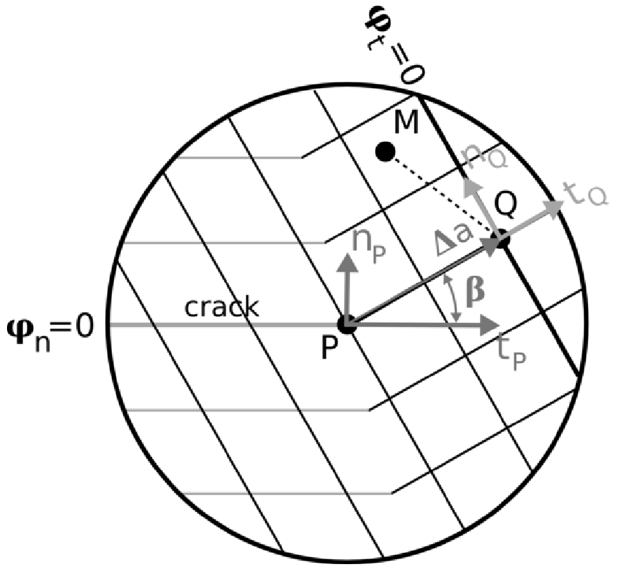
Figure 6.1-1 : iso-surfaces of the two level-sets obtained by the standard update process, with reset and reorthogonalization. \(P\) is a point at the bottom of a 3D crack. \(Q\) is the new position of this point after an advance of \(\Delta a\) with a propagation angle \(\beta\) .
We consider point \(M\) in the field of calculation where we must calculate the new value of the two level-sets. We project this point onto the bottom of the crack using the same algorithm as that described in paragraph 2.2 and we obtain the point \(P\) (figure). The local base \(({t}_{P},{n}_{P})\) and the advance speed \({V}_{P}\) at point \(P\) can be calculated as described in paragraphs 2.2, 2.3, and 2.4. For the angle of propagation, we use the same linear interpolation as that used for the speed (see paragraph § 2.2 and figure:
The advance of the crack at point \(P\) at the bottom can therefore be easily calculated:
Where \(\Delta t\) is the time or, in equivalent terms, the number of fatigue cycles to be simulated at the current propagation step (see discussion of paragraph 3.1).
The new position \(Q\) of the bottom point \(P\) can therefore be calculated like this:
Where \(O\) is the origin point of the global base in which the coordinates of the points are expressed.
Finally, the base at point \(Q\) can be calculated by an angle rotation from the base to the point P around the axis normal to the plane \({t}_{P}\mathrm{-}{n}_{P}\):
All the ingredients for calculating level-sets are now known. We can therefore use the same equations as those used in paragraph 5.2:
In order to preserve the existing surface of the crack (iso-surfaces in gray in the figure), the calculation of the normal level-set with the equation above is done only at the points in the domain where \({\mathrm{\varphi }}_{t}(\text{M})>0\).
6.2. Treatment of problem areas#
The equations written in the previous paragraph apply if the vector \(\overrightarrow{\text{PM}}\) is in the \({t}_{P}\mathrm{-}{n}_{P}\) plane (figure) (bib 18). This is not the case for all points that do not have a normal projection point on the bottom of the crack. In this case, an end point of the background is selected as the projected point P by the projection algorithm described in paragraph 2.2.
These problem points can be treated by rotating the base \(({t}_{P},{n}_{P})\) which makes it possible to re-establish the coplanarity condition of the plane \({t}_{P}\mathrm{-}{n}_{P}\) and the vector \(\overrightarrow{\text{PM}}\) or \(\overrightarrow{\text{QM}}\) (bib 18).
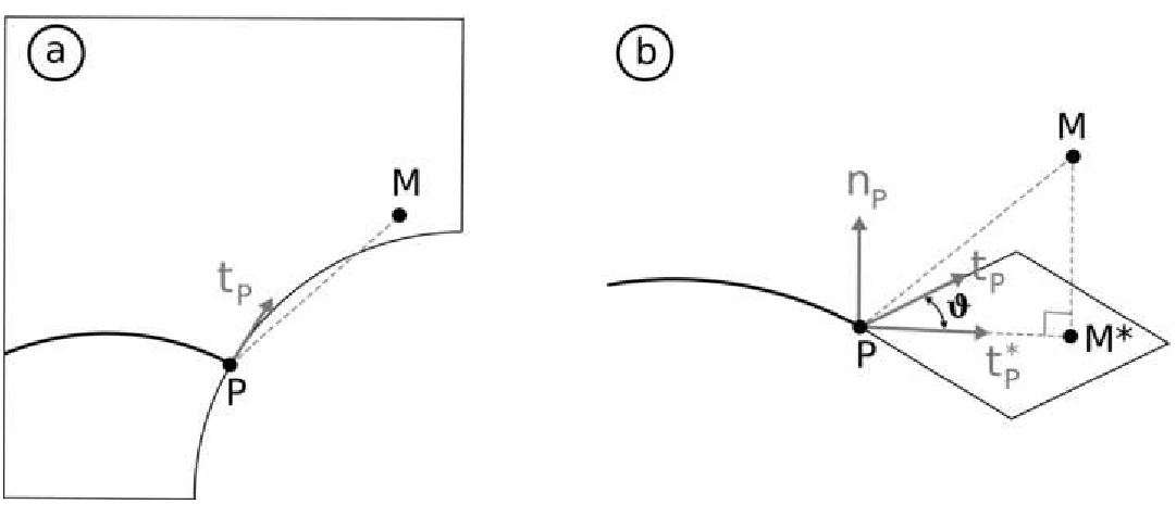
Figure 6.2-1 : a) example of a problem point. b) rotation from base to point \(P\) to restore the coplanarity condition between the plane \({t}_{P}\mathrm{-}{n}_{P}\) and the vectors \(\overrightarrow{\text{PM}}\) or \(\overrightarrow{\text{QM}}\) .
An example of a problem point can be seen in figure a. To re-establish the coplanarity condition, it is possible to rotate \(\theta\) of the base \(({t}_{P},{n}_{P})\) around the vector \({n}_{P}\) in such a way that the plane \({t}_{P}^{\text{*}}\mathrm{-}{n}_{P}\) contains the point \(M\) (figure b). In fact, in this way the new position of the point \(P\) after propagation (point \(Q\) in the figure) is contained in the plane \({t}_{P}^{\text{*}}\mathrm{-}{n}_{P}\), which makes it possible to verify the coplanarity condition.
The new vector \({t}_{\text{P}}^{\text{*}}\) can be calculated from the projection \({M}^{\text{*}}\) of the point \(M\) on the plane normal to the axis \({n}_{P}\) (figure b). First, we calculate:
: label: eq-61
vec {{text {M}}} ^ {text {*}}}text {*}}}text {*}}}text {M}} ^ {text {M}} ^ {text {*}}}}right)cdot {n}} =left (vec {text {P}}}cdot {n}}}cdot {n}} _ {text {n}} _ {text {N}} _ {text {N}} _ {text {P}} _ {text {P}} _ {text {P}}
This makes it possible to obtain the new vector:
: label: eq-62
{t} _ {text {P}}} ^ {text {*}}}mathrm {*}}mathrm {=}frac {overrightarrow {text {PM}}}mathrm {-}}overrightarrow {{text {*}}}mathrm {parallel}overrightarrow {parallel}overrightarrow {parallel}overrightarrow {M}}} {mathrm {parallel}overrightarrow {parallel}overrightarrow {text {PM}}mathrm {parallel}mathrm {-}mathrm {-}mathrm {parallel}overrightarrow {{text {M}}} ^ {text {*}}}text {*}}}text {*}}}text {M}}text {M}}
To correctly take into account the sign of the tangent level-set, the vector \({t}_{\text{P}}^{\text{*}}\) must be reoriented in the direction given by \({t}_{\text{P}}\) (bib 18):
If the two vectors \({t}_{\text{P}}^{\text{*}}\) and \({t}_{\text{P}}\) are orthogonal, the above equation cannot be applied but we can write right away that:
Using the vector \({t}_{\text{P}}^{\text{'}}\) in place of \({t}_{\text{P}}\) in the equations in paragraph § 6.1 makes it possible to properly calculate the level-sets for the problem points.
6.3. Normal level-set discontinuity and calculation limitations#
Computing the normal level-set only at points \(M\) for which \({\mathrm{\varphi }}_{t}(\text{M})>0\) results in a discontinuity in the normal level-set, as shown in (bib 18). The situation is shown in figure. The normal level-set was not recalculated in the gray colored area, implying an iso-surface discontinuity between the gray area and the area where the level-set was recalculated.
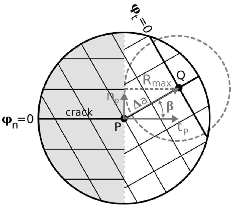
Figure 6.3-1 : discontinuity of the iso-surfaces of the normal level-set and maximum radius \({R}_{\mathit{max}}\) from the calculation domain of CALC_G to be used. As demonstrated in (bib 18), this discontinuity does not cause any problem for X- FEM calculations (identification of new cut cells in particular). In addition, the iso-zero continuity of the normal level-set is maintained, which ensures the continuity of the crack surface. The only condition to be met to manage this discontinuity concerns the maximum value of the calculation radius of CALC_G (see U4.82.03). The purpose of this condition is to prevent the field of calculation of CALC_Gcontienne from discontinuity (gray circle in the figure):
Where we take the maximum value of \(\Delta a\) and \(\beta\) along the bottom of the crack.
Although it restricts the propagation angle to values strictly less than \(\pi /2\) (under penalty of increasing refinement as we get closer to \(\pi /2\)), this condition is not very restrictive because it is advisable to respect a similar relationship even in the case of updating level-sets using the simplex or upwind method.
6.4. Domain location#
As shown in (bib 18), the location of the domain described in paragraph § 5 is no longer necessary if using the direct calculation of level-sets.
First, locating the domain would not improve the robustness of the algorithm. In (bib 14), it is shown that small errors in calculating the propagation angle (which is always the case during numerical simulations) are amplified at points located far from the crack front (due to the linear interpolation used to create the \({V}_{N}\) speed field). The iso-surfaces of the normal level-set are then no longer regular and this can lead to the failure of the level-set reset phases. Localizing the domain thus makes it possible to reduce the level-set update domain to a domain encompassing the crack front, which leads to a limitation of the amplification effect. However, the geometric method successfully manages non-regular iso-surfaces since it is based on explicit polynomial equations and not on differential equations. In addition, the geometric method does not use a process for resetting and reorthogonalizing the level-sets (which are calculated at each propagation step). For all these reasons, the location of the domain does not affect the robustness of the geometric method.
Localizing the domain when using the geometric method would also not necessarily reduce the calculation time required to update the level-sets. It turns out that the calculation of the level-sets at each point in the domain is fast and that the time required for this calculation may be less than the time required to select the points in the localized domain. The algorithm used for the selection of points belonging to the restricted domain is based on the calculation of the distance between a point \(M\) in the domain and its projected \(P\) on the crack front. As point \(P\) must also be calculated for the calculation of the level-sets, the additional calculation cost for the selection algorithm is reduced to the cost of calculating the distance \(∣∣\vec{\mathit{PM}}∣∣\) and the complexity of the algorithm is \(O(n)\). Even if the complexity of the algorithm for updating level-sets by the geometric method is \(O(n)\), it seems clear that the sum of the calculations performed by the selection algorithm will be less than that performed by the algorithm for updating level-sets. This leads one to think at first glance that the location of the domain would be advantageous in terms of calculation time compared to the calculation of level-sets throughout the domain. However, the selection (based on distance \(∣∣\vec{\mathit{PM}}∣∣\)) of points within the restricted domain is not sufficient. In fact, to calculate the local base at each point, it is a question of determining the gradient of the level-sets, which requires the selection of the elements containing the selected points (the shape functions of the elements being used to calculate the gradients). Even if the selection algorithm does not necessarily change, the number of operations performed increases and this may make the selection calculation time longer than the calculation of level-sets by the geometric method throughout the domain. Note that, at the same time, the time to calculate the gradients of the level-sets is also longer if the location of the domain is not taken into account.
Finally, the advantage of the location of the domain in terms of calculation time depends strongly on the algorithms and implementations chosen and on the number of points in the calculation domain. The location of the domain could thus be advantageous in the case of « very large » finite element meshes. In this case, limiting the updating of level-sets to a group of nodes (fixed and defined by the user) defining the potential surface for propagation of the crack may be a more effective way to reduce calculation time rather than choosing a domain location algorithm for which a new restricted domain must be calculated at each propagation step in order to follow the displacement of the crack front.