5. Location of the level-set calculation domain#
In paragraph [§ 4.2.1.5] it was said that, in the case of using an auxiliary grid for the upwind method, the values of the level-sets are updated, reset, and reorthogonalized for all points in the grid but that only the values in a region around the bottom of the crack are projected onto the mesh of the structure. This shows that the updating of the level-sets, their resetting and their reorthogonalization are necessary only in the region around the bottom of the crack, regardless of whether or not an auxiliary grid is used, and that the domain already defined for the projection between auxiliary grid and structure mesh ([§ 4.2.1.5]) can also be used to locate the calculation domain. An advantage of this location is obviously that the calculation time required for updating and resetting the level-sets is less compared to the case where all the nodes and elements of the mesh or the auxiliary grid are used. In fact, in the case where the level-sets are updated at nodes/points that are very far from the bottom of the crack in the presence of oscillations in the angle and the speed of propagation between successive points at the bottom of the crack, the iso-zeros of the normal level-set can present very marked irregularities because of the linear variation imposed at the normal speed ([§ 2.5]). An illustrative example is shown figure and figure. It shows a 3D crack propagating in mixed mode at an angle of propagation that changes linearly along the bottom of the crack. Small disturbances have been superimposed on the expected theoretical value, so that the variation in the angle of propagation with the position on the background is not perfectly linear (figure). These disturbances simulate the presence of small errors in a numerical calculation of angle values.
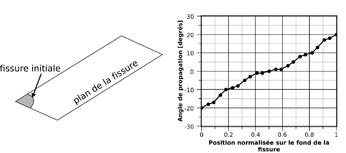
Figure 5-1 : initial configuration (left) of the simulation of an out-of-plane propagation of a 3D crack at an angle of propagation that changes almost linearly with respect to the position considered on the bottom of the crack (graph on the right) .
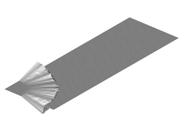
Even if the disturbances in the angle of propagation, and therefore in the normal speed, are small, they are amplified by the linear variation imposed on this speed component in the calculation domain, which is very clear if we visualize the iso-zero of the normal level-set after the only update phase (figure). The location of the calculation domain makes it possible to limit this effect (figure).
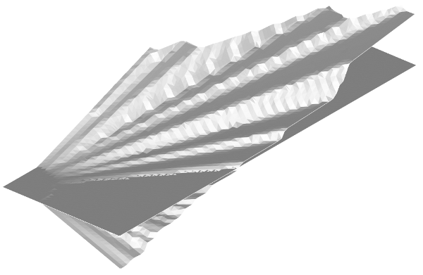
Figure 5-2 : iso-zero of the normal level-set after the only update phase. The angle of propagation in figure has been imposed. The plane of the initial crack has been superimposed for comparison.
Figure 5-3 : iso-zero of the normal level-set obtained with an update domain restriction compared to that in figure *. It should be noted that for this figure the plane of the initial crack has not been represented, contrary to what was done for Figure*** . We can therefore conclude that the value of the level-set has not been changed for points outside the calculation domain.
5.1. Selection of nodes/points and elements of the localized computing domain#
The domain to be used for the location is the one already defined for the projection between the auxiliary grid and the mesh of the structure ([§ 4.2.1.5]). In fact, this domain is extended to all the points used for mechanical calculations and it makes it possible to preserve the surface of the existing crack, as already shown (figure). The methods will be applied only to the nodes and elements contained in this field, which is defined by circle 3 in figure. In 3D, this domain coincides with a torus built around the bottom of the crack and whose radius is equal to that of circle 3. In all cases the radius of the localized domain is therefore equal to:
\({R}_{\mathit{loc}}\mathrm{=}\Delta a+{R}_{\mathit{calc}G}\)
where \(\Delta a\) is the advance of the crack to be imposed (chosen by the user) and \({R}_{\mathit{calcG}}\) is the radius of the domain used by CALC_G.
We can therefore first select the nodes of the grid or the mesh that have a distance from the bottom of the crack less than or equal to \({R}_{\mathit{loc}}\) (figure on the left). This distance can be calculated very quickly because for each node we already know its projection on the crack background ([§ 2.2]). Then we take all the elements that have at least one of the nodes selected previously (gray elements in the figure on the right). This makes it possible to correctly select all elements that are cut by the domain border and are therefore partially contained within the domain. In this way, the entire area (or volume in 3D) of the domain is correctly covered by the selected elements. Finally, the list of domain nodes must be updated by adding the nodes of the elements partially contained in the domain (nodes marked with a small circle in the figure on the right). The quickest and easiest way to do this is to rebuild the list by taking all the nodes of the selected items. Once the list of nodes has been updated, the value of radius \({R}_{\mathit{loc}}\) of the discretized domain, that is, of the domain constituted by the nodes and the selected elements, must be updated by taking the value at the node of the discretized domain farthest from the bottom. This operation is necessary for the next part ([§ 5.3]).
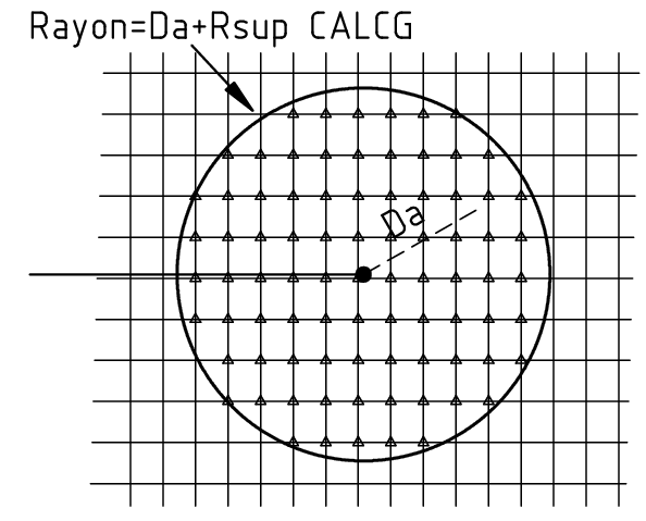
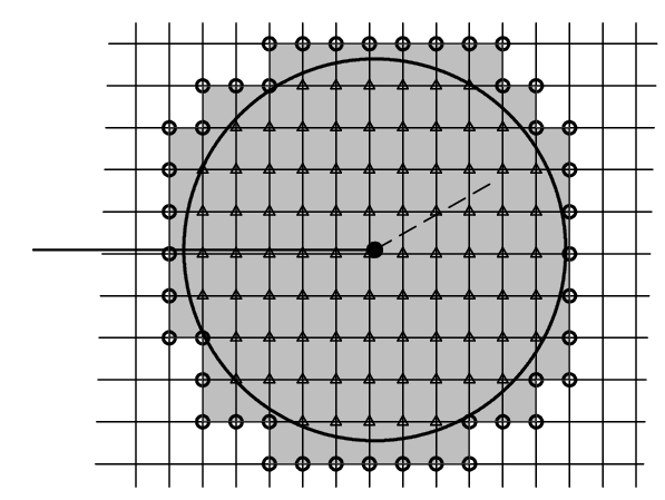
Figure 5.1-1 : example of selecting nodes and elements of the location domain. It is assumed that this domain coincides with the circle in the figure. The first step (on the left) is selecting nodes at a distance less than or equal to \({R}_{\mathit{loc}}\) . The selected nodes are marked with a small triangle. Then the elements that contain at least one of these nodes in their definition are selected (gray elements on the right). Finally, we select all the nodes of the elements that were taken: the nodes marked with small circles are added to those that were selected at the beginning.
5.2. Displacement of the localized domain following the propagation of the crack#
Level-sets are updated and reset exclusively at the nodes that define the localized domain (nodes marked with triangles and circles in the figure on the right). This means that the level-set values at nodes outside of the localized domain are not changed, which causes problems during successive propagation steps. The situation is illustrated figure for a point \({P}_{1}\) in plane \(t\mathrm{-}n\) (plane \({e}_{1}\mathrm{-}{e}_{2}\) in the figure). At the beginning of the propagation the bottom of the crack coincides with the point \({P}_{1}\) and the localized domain with the circle \({\Omega }_{1}\). To simulate the spread, the level-sets are updated and reset only in this circle. The new bottom position after the first propagation step coincides with \({P}_{2}\). At the second propagation step, the bottom of the crack coincides with point \({P}_{2}\) and a new \({\Omega }_{2}\) domain is built around this point for updating and reinitializing the level-sets. The value of the level-sets has not been updated to the previous propagation step for all the points in \({\Omega }_{2}\): only the level-sets of the points in \({\Omega }_{2}\) in common with \({\Omega }_{1}\) are up to date (points on the gray surface of the figure). For all other points, the value of the level-sets is the value we had at the start of the spread. The correct values at these other points must therefore be calculated at the start of the second propagation step.
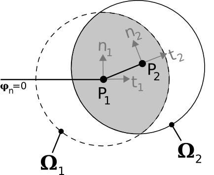
Figure 5.2-1 : displacement of the localized domain between two successive propagation steps. The bottom of the crack moves from \({P}_{1}\) to \({P}_{2}\) .
The calculation of the correct level-set values for all the points in the white region in the white region of domain \({\Omega }_{2}\) of the figure can be done using the signed distance definition of the level-sets (bib 14). For each point \(M\) in this region (figure), the level-sets can be calculated like this:
\({\varphi }_{n}(\text{M})=\overrightarrow{\text{M}{\text{P}}_{2}}\cdot {n}_{2}\)
\({\varphi }_{t}(\text{M})=\overrightarrow{\text{M}{\text{P}}_{2}}\cdot {t}_{2}\)
These equations allow you to calculate the correct value of the level-sets with the right sign. It should be noted that, in the 3D case, point \({P}_{2}\) is the point projected from point \(M\) on the bottom of the crack. For each point \(M\), its projection and the base \({n}_{2}\mathrm{-}{t}_{2}\) have already been calculated during the phase of extending the speed from the bottom of the crack to the points in the calculation domain ([§ 2.2]). All the ingredients for the calculation are therefore already available and for each point \(M\) the evaluation of the correct level-set is limited to the calculation of two dot products, which is very quick to do.
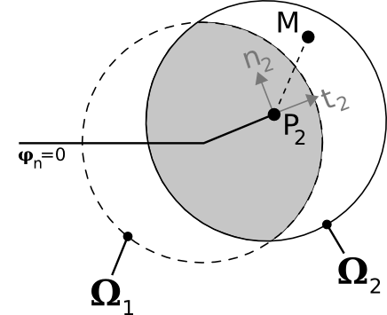
Figure 5.2-2 : calculation of the correct values of the level-sets at the points of \({\Omega }_{2}\) that are outside the domain \({\Omega }_{1}\) of the previous propagation step. The calculation is done at the very beginning of the current propagation, i.e. before the level-sets are updated and reset.
It should be noted that even if the values of the level-sets calculated by the equations above are not very precise, the update phase is only used to initialize them and the good level-sets will be recovered by the reset phases.
5.3. Limitations on the value of the radius of the localized domain between two successive propagations#
The equations given in paragraph 33 for calculating the correct level-set values can only be applied to the points for which the \({n}_{2}\mathrm{-}{t}_{2}\) base is valid for calculating the signed distance. This means that point \(M\) must belong to the half-plane shown in figure, which contains the base \({n}_{2}\mathrm{-}{t}_{2}\), the bottom of the crack \({P}_{2}\) and whose edge is a line normal to the edge connecting \({P}_{1}\) and \({P}_{2}\) parallel to \({n}_{2}\).
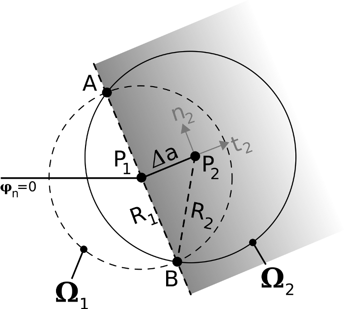
Figure 5.3-1 : definition of the half-plane to which the point \(M\) in the figure must belong in order for the level-set calculation equations in paragraph 33 to be valid.
This condition on the position of the point \(M\) results in a condition on the maximum value of the radius \({R}_{2}\) of the domain \({\Omega }_{2}\): the maximum value is the one for which the two intersection points (\(A\) and \(B\)) between the two domains \({\Omega }_{1}\) and \({\Omega }_{2}\) are on the edge of the half-plane of validity of the equations, as shown in figure. These two points are always symmetric with respect to the edge connecting \({P}_{1}\) and \({P}_{2}\). The maximum value of radius \({R}_{2}\) can therefore be easily calculated:
\({R}_{2}\le \sqrt{\Delta {a}^{2}+{R}_{1}^{2}}\)
The value of the radius of the current domain is therefore limited by the values of the advance of the crack and the radius of the domain used at the previous propagation step. Normally there is no point in changing the value of the domain radius between two successive propagations. In this case, as \({R}_{1}\) is equal to \({R}_{2}\), the inequality on \({R}_{2}\) is necessarily true regardless of the value of the advance chosen.
However, it should be noted that the value of the domain radius may change compared to the theoretical value given by the user due to the discretization of the domain ([§ 5.1] and figure on the right). So, even if we give \({R}_{2}\mathrm{=}{R}_{1}\) to the current propagation step, the effective value of the domain radius will be as follows:
\({R}_{2\text{eff}}\mathrm{=}{R}_{2}+\Delta {R}_{2}\mathrm{=}{R}_{1}+\Delta {R}_{2}\)
where \(\Delta {R}_{2}\) is the increment of the radius \({R}_{2}\) due to the discretization of the domain, which is of the order of the average length of the edges of the elements around the border of the localized domain (see figure).
For the same reason, the effective value of radius \({R}_{1}\) at the previous propagation step may be different from the theoretical value given by the user:
\({R}_{1\text{eff}}\mathrm{=}{R}_{1}+\Delta {R}_{1}\)
where \(\Delta {R}_{1}\) is the increment of the radius \({R}_{1}\) due to the discretization of the domain, which is of the order of the average length of the edges of the elements around the border of the domain located at the previous propagation step.
So the inequality above can be written in the following form:
\({R}_{1}+\Delta {R}_{2}\mathrm{\le }\sqrt{\Delta {a}^{2}+{({R}_{1}+\Delta {R}_{1})}^{2}}\)
In the case where the length of the edges of the auxiliary grid used is uniform in the field, \(\Delta {R}_{2}\mathrm{\approx }\Delta {R}_{1}\), and the inequality is always verified. On the other hand, if this length changes in the domain, we could have \(\Delta {R}_{2}>\Delta {R}_{1}\) and the inequality could not be verified.
In the latter case, it is necessary to refine the mesh (or the auxiliary grid) to reduce the difference between \(\Delta {R}_{1}\) and \(\Delta {R}_{2}\) or use a higher \(\Delta a\) crack extension.