4. Resetting and reorthogonalizing level-sets#
4.1. Introduction#
During their evolution, level-sets must imperatively keep a definition relatively close to signed distance functions.
The first reason is the calculation of stress intensity factors at the bottom of the crack by the \(G\) -Theta method, for which the polar coordinates \((r,\theta )\) are defined in the local base as \(r=\sqrt{{\text{lsn}}^{2}+{\text{lst}}^{2}}\) and \(\theta =\text{arctan}(\text{lsn}/\text{lst})\); the use of signed distances for the calculation of polar coordinates is therefore necessary.
In addition, during crack propagation, the updating equation presented above (paragraph [§:ref: 3 <Ref141586894>]) involves the norms of the gradients of the level-sets, which must remain sufficiently close to unity, because if:math: | |nablamathrm {varphi} | does not equal: 1, the crack does not advance with the speed: 1, because if:math: | | | |nablamathrm {varphi} | does not equal :math: 1, the crack does not advance with the speed:: math:` {V} _ {mathrm {varphi}} `defined.
After the update phase, level-sets sometimes lose their sense of signed distance function, especially in the case of out-of-plane propagation (case of a solicitation where \({K}_{\mathit{II}}\mathrm{\ne }0\)), which introduces normal speed (see Figure 4.1-1).
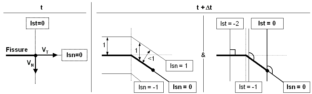
Figure 4.1-1 : Propagation of level-sets and loss of signed distance and orthogonality function
After propagation it is therefore necessary to go through a stage called « reset » whose aim will be to minimize \(∣∣\nabla \mathrm{lsn}∣-1∣\) and, \(∣∣\nabla \mathrm{lst}∣-1∣\) as well as a « reorthogonalization » step whose objective will be to minimize \(\mathrm{\mid }\mathrm{\nabla }\text{lsn}\text{.}\mathrm{\nabla }\text{lst}\mathrm{\mid }\). In fact, level-sets are only rigorously defined if, at any point in space, \(\mid \nabla \text{lsn}\mid =1\), \(\mid \nabla \text{lst}\mid =1\) and \(\nabla \text{lsn}\text{.}\nabla \text{lst}=0\).
However, in the case of a non-planar crack, it is impossible to have two functions whose gradients are orthogonal to each other and unit norms at any point in space. The antagonism between the two properties appears on Figure 4.1-2, on which a function \(\mathit{lst}\), which is either normalized or orthogonal, is defined, starting from an iso-zero of \(\mathit{lsn}\).
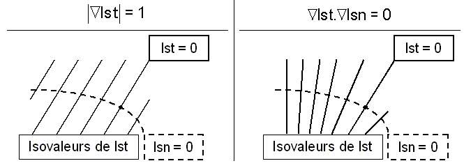
Figure 4.1-2 : Antagonism Initialization - Orthogonalization
It is therefore necessary to give priority to one or the other of these properties. Given the main use of these functions for the \(G\) -Theta method, it seems more important that the gradients be well normalized, rather than orthogonal, so that the \((r,\theta )\) polar coordinates make sense. In order to have an orthonormal local base, it is also necessary on the crack background that the gradients be standardized and orthogonal. The sequence of steps proposed in (bib 1) is therefore:
reset \(\mathit{lsn}\):
The iso-zero of \(\mathit{lsn}\), which is of major importance for the definition of crack, is unchanged;
reorthogonalization of \(\mathit{lst}\) with respect to \(\mathit{lsn}\) fixed:
\(\mathit{lst}\) is straightened compared to \(\mathit{lsn}\) without modifying the bottom of the crack \((\text{lsn}=0)\cap (\text{lst}=0)\);
reset \(\mathit{lst}\):
Level-set \(\mathit{lst}\) is initialized with respect to its iso-zero having been orthogonalized.
4.2. Resolution by the fast marching method#
In the following we will analyze two methods for resetting and reorthogonalizing level-sets. The first method (« Upwind » method) can only be applied to rectangular elements in 2D and hexahedra in 3D only, an extension to all types of meshes being possible with the use of an auxiliary grid. The second method (« Simplex » method) can be applied only to simplex elements (triangles in 2D and tetrahedra in 3D), a cut of the meshes going beyond this framework making it possible to use this method with all types of meshes.
4.2.1. « Upwind » method#
We saw previously that after the propagation phase of a level-set, it was necessary to reset it in order to maintain a signed distance function. In other words, if we assume that the function:math: mathrm {varphi} (vec {x}, t=0) = {mathrm {varphi}} _ {0} (vec {x}) checks for each node in the mesh the property of a signed distance function given by:math: left|nablamathrm {varphi}}}right|=1, the level-set function at:math: t>0 no longer has this property. It is therefore necessary to set up a reset process allowing to:math: mathrm {varphi} to become a signed distance function again.
Here we propose a fast-marching method introduced by Sethian [19], which solves the eikonal equation of the form:
:math:`begin{array}{c}left |
nabla mathrm{varphi }(x)right |
=F(x),xin mathrm{Omega }\ mathrm{varphi }(x)=0,xin partial mathrm{Omega }end{array}` |
With \(\mathrm{\Omega }\in {\mathrm{ℝ}}^{n}\), \(n\text{}\text{}\in \{\mathrm{2,3}\}\), and \(F\) a function with positive values.
The point we’re interested in here is just one particular case of this equation: when \(F=1\). The solution thus gives the \(\mathrm{\varphi }\) signed distance function.
The principle of the fast-marching method consists in propagating the data on the distance of the points from the lowest values, that is to say close to the interface, to the most distant zones, from one step to the other.
For the propagation of level-sets, values around \(\mathit{ls}=0\) are used to propagate information. Two calls to the method are required to process all the nodes in the mesh: the first call will deal with the positive points of the level-set and the second the negative points.
To do this, the method divides the mesh nodes into three categories:
Frozen points: region of the mesh where the points have already been calculated (black circles);
Narrow band: region close to the points already calculated (gray band);
Far away: set of the remaining points (white circles).
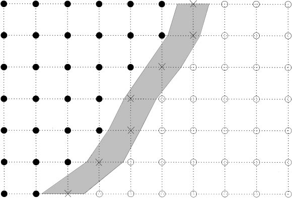
Figure 4.2-1: distribution of mesh nodes The fast-marching method can do without the reorthogonalization step because once \(\mathit{lsn}\) has been reset, you can initialize the values of lst to its non-reorthogonalized iso-zero by taking the values at the nodes obtained by a geometric calculation. We can therefore use these values as the initial condition of the method to propagate this exact information about \(\mathit{lst}\) to the entire domain.
4.2.1.1. Discretization of the problem#
In the reinitialization phase of a level-set, we seek to solve numerically a particular case of the eikonal equation:
: label: eq-32
===nablaphi =1
If we note \({\mathrm{\Delta }}_{x}\) \({\mathrm{\Delta }}_{Y}\) and \({\Delta }_{Z}\) the space steps in \(x\), \(y\) and \(z\), an upwind discretization by finite difference of this equation is:
With:
We are looking for the solutions of the quadratic trinomial that approximates equation () in the form:
with:
: label: EQ-None
p ({mathrm {varphi}}} _ {i, j, k}) = {left (frac {{mathrm {varphi}} _ {i, j, k} - {mathrm {varphi}} _ {varphi}}} _ {varphi}}} _ {varphi}}} - {mathrm {varphi}}} - {varphi}} _ {varphi}} - {mathrm {varphi}}} - {varphi}} _ {varphi}} - {mathrm {varphi}}} - {varphi}} _ {varphi}} - {mathrm {varphi}}} _ {varphi}} - {(frac {{mathrm {varphi}}} _ {i, j, k}} - {mathrm {varphi}} _ {2}} {{mathrm {Delta}}} _ {y}}right)} _ {y}}}right)}}} ^ {2} + {2} + {left (frac {{mathrm {varphi}}} _ {i, j, k}} _ {y}}} _ {y}}}right)}} ^ {2} + {2} + {left (frac {{mathrm {varphi}}} _ {i, j, k}} - {right)}}} _ {i, j, k} - {right)}}}mathrm {varphi}} _ {3}}} {{mathrm {Delta}} _ {z}}right)} ^ {2} -1
The two solutions of () are:
The distance increases as we move away from the interface. Solution \({\mathrm{\varphi }}_{i,j,k}\) is evaluated at a point further away from the interface than the points at distances \({\mathrm{\varphi }}_{1}\), \({\mathrm{\varphi }}_{2}\), and \({\mathrm{\varphi }}_{3}\). So we necessarily have only \({\mathrm{\varphi }}_{i,j,k}>{\mathrm{\varphi }}_{1}\), \({\mathrm{\varphi }}_{i,j,k}>{\mathrm{\varphi }}_{2}\), and \({\mathrm{\varphi }}_{i,j,k}>{\mathrm{\varphi }}_{3}\). However, we have:
This involves:
So the solution () is necessarily the only acceptable one.
4.2.1.2. Method implementation#
The numerical discretization of equation () by finite difference upwind is only applicable on hexahedral meshes (or rectangular in 2D) whose edges are well oriented in three directions \(({j}_{1},{j}_{2},{j}_{3})\) forming a base of \({\mathrm{ℝ}}^{3}\) .As for the upwind method, an auxiliary grid is used to extend the method to irregular meshes.
Here we present only an algorithm for the positive \(\mathrm{\varphi }\) case (\(\mathit{lsn}>0\) or \(\mathit{lst}>0\)), a simple multiplication by \(-1\) of this function making it possible to treat the other side of the level-set.
The algorithm put in place is as follows:
Initialization
We identify the knots for which \(\mathit{ls}\ge 0\)
We identify the points close to \(\mathit{ls}=0\) and \(\mathit{ls}\ge 0\), that is to say the knots (narrow band) of the stitches cut by \(\mathit{ls}=0\), such as \(\mathit{ls}\ge 0\)
Note: Since we want to propagate the calculation to remote areas, we must first ensure that these points provide consistent initialization from the point of view of a distance function. On performs a geometric calculation of the level-sets on the elements cut by \(\mathit{ls}=0\). **We assign the other positive nodes of the value* \(+\infty\). They will belong to the set **far, while the negative points will be included in a third set* **known.*
Loop
As long as a node has \(\mathit{ls}\ge 0\), we locate the node with the lowest value of \(\mathrm{\varphi }\) in the narrowband.
For each node around this minimum, we get \({\mathrm{\varphi }}_{1}\), \({\mathrm{\varphi }}_{2}\), and \({\mathrm{\varphi }}_{3}\) as defined by ().
Figure 4.2-2: Neighborhood of the node to be calculated For each node around the minimum, its value is calculated by the explicit formula ().
End of the loop
4.2.1.3. Fast marching and the geometric method#
Problem nodes
To perform the calculations using the fast-marching method, equation () was discretized by finite differences. To calculate the value of a node, it is therefore necessary to have the information necessary to apply the explicit formula (). For each calculated node, we must have retrieved \({\mathrm{\varphi }}_{1}\), \({\mathrm{\varphi }}_{2}\) and \({\mathrm{\varphi }}_{3}\) beforehand: if these values exist then the calculation by the formula () is immediate. In the opposite case, i.e. if \({\mathrm{\varphi }}_{1}=+\mathrm{\infty }\) or \({\mathrm{\varphi }}_{2}=+\mathrm{\infty }\) or \({\mathrm{\varphi }}_{3}=+\mathrm{\infty }\), we cannot apply the formula () because the lack of information will cause equation () to be incorrectly approximated.
To solve this problem, one can use the geometric method for the problem node by directly calculating its value. A simple test in the code thus makes it possible to know whether the point to be calculated is evaluated by the fast-marching method or by the geometric method. To avoid possible problems, it is a good idea to also test the sign of the value under the root in the formula ().
So if:
The calculation by the formula () is legal. Whereas if:
The formula () is no longer valid and a geometric calculation on this node is required.
Resetting lst
Once \(\mathit{lsn}\) has been reset using the fast marching method, we move on to resetting \(\mathit{lst}\) without going through the reorthogonalization step. The main problem for this stage is that the iso-zero in \(\mathit{lst}\) is not orthogonal to the iso-zero in \(\mathit{lsn}\). Since fast marching is only applicable under the condition that the distance increases away from the interface, we can start the method around the iso-zero of the non-orthogonalized \(\mathit{lst}\) by performing a geometric calculation for these nodes in order to retrieve the right values and propagate the information as defined above. The method will thus reorthogonalize \(\mathit{lst}\) and assign it the signed distance function property in a single calculation. To increase the precision and the location of the crack bottom, two LST resets will be performed in a row. The first reset allows the iso-zero to be moved so that it becomes orthogonal to \(\mathit{lsn}\) and the second will increase the precision in locating the crack bottom. The problem may come from the iso-zero position of \(\mathit{lst}\) before the first reset. If this position is too far from the new position after resetting, a less precise location of the crack base is observed. With two steps, we ensure that the localization of the iso-zero of \(\mathit{lst}\) will not disturb the solution.
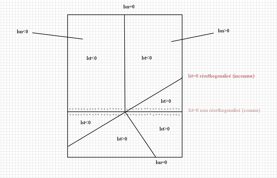
Figure 4.2-3: Resetting \(\mathit{lst}\)
4.2.1.4. Applying the upwind method to an irregular mesh#
For the application of the finite differences method, we must use a very regular mesh, consisting of hexahedral cells in 3D and rectangular cells in 2D, whose edges are well oriented according to the directions of the base of space \({\mathrm{ℝ}}^{3}\) in 3D and \({\mathrm{ℝ}}^{2}\) in 2D. This represents a very strong restriction for creating the mesh and therefore excessively limits the cases that can be treated by the method.
One solution to this problem is to use two different meshes (bib 12): one mesh is used for the physical structure (physical mesh) and one mesh is used for the representation of the level-sets (level-sets mesh). The restrictions of the finite difference method apply only to this last mesh. The values of the level-sets on the physical mesh can be calculated by projecting the known values onto the level-sets mesh. This is necessary for the location of the bottom of the crack in the physical mesh. In fact, fracture mechanics calculations are carried out only on this last mesh. It is therefore possible to update, reset and reorthogonalize level-sets using only the level-sets mesh. Then we can project the level-sets onto the physical mesh from the level-sets mesh. Finally, it is possible to calculate the stress intensity factors and the direction of propagation of the crack using only the physical mesh.
The projection also makes it possible to obtain geometric independence between the two meshes: the level-set mesh does not need to be oriented according to the directions of the base chosen for the physical mesh and it can only occupy the volume of the crack propagation zone in the structure.
The nodes of the level-set mesh, constructed as described above, therefore constitute a cloud of points aligned in three orthogonal directions. The grid formed by these points can be used to apply the « upwind » method. In the rest of this document and in the Code_Aster syntax, the expression auxiliary grid will be used to indicate all of these points. Also, to simplify the notations used and to make them clearer, we will simply use the term mesh to indicate the physical mesh.
4.2.1.5. Implementation of the projection between the auxiliary grid and the physical mesh#
In Code_Aster the auxiliary grid is not given as a set of well-oriented points but as a mesh and therefore some intermediate steps are necessary to apply the upwind finite difference method. In fact, for this method all the points of the grid, taken to be coincident with the nodes of the given level-set mesh, must be arranged according to the directions of a local base. We must therefore calculate this local base and then we must order the nodes and calculate the distance between two successive nodes.
The local base calculation is very easy because you can use the definition of the grid elements of the auxiliary grid. In fact, the edges of the elements are well oriented with respect to the axes of a local base and this base can be defined by taking edges that are orthogonal to each other. In addition, we are only looking for the direction of the axes of the local base. You can therefore use the edges of any element of the mesh. In 3D, the first element of the mesh of the auxiliary grid makes it possible to determine, from one of its nodes, the three edges that lead to it, and thus to calculate the three unit vectors in the three directions of the selected edges. In 2D we do the same operation with two edges.
For the ranking of the nodes according to the directions of the axes of the calculated local base, you can once again use the edges of the elements. For each node in the mesh, you can select the elements that contain it. For each of the selected elements, the edges that start from the node are selected. Finally, for each of the selected edges, the points are ordered according to one of the directions of the local base of the mesh using the dot product between the edge and the unit vectors of the local base and the distance between the nodes of the edge can be calculated. In 3D the algorithm put in place is as follows (all the vectors are represented in the base chosen to represent the nodes of the physical mesh):
We identify the three unit vectors of the local base: \({j}_{1}\), \({j}_{2}\) and \({j}_{3}\)
Loop on the \(N\) nodes of the mesh
We initialize to zero the stored values of the six nodes that are connected (successive or previous) to node \(N\) according to the three unit vectors of the local base
We identify the elements that include node \(N\) in their definition
Loop over selected items
We identify the three edges that start from node \(N\)
Loop on the three selected edges
We calculate the \(\overrightarrow{\mathit{NA}}\) vector between the two end nodes of the edge. This vector is oriented in the direction that goes from node \(N\) to the other node \(A\) end of the edge.
We calculate the components of vector \(\overrightarrow{\mathit{NA}}\) according to the local base:
\({\mathit{NA}}_{1}=\vec{\mathit{NA}}\cdot {j}_{1}\)
\({\mathit{NA}}_{2}\mathrm{=}\overrightarrow{\mathit{NA}}\mathrm{\cdot }{j}_{2}\)
\({\mathit{NA}}_{3}\mathrm{=}\overrightarrow{\mathit{NA}}\mathrm{\cdot }{j}_{3}\)
The tolerance is calculated which is used to check if a component is zero. This value is calculated as a percentage :math:`p` (set to 1% in*Code_Aster) of the vector length:
\({l}_{\mathit{max}}\mathrm{=}p\mathrm{\cdot }∣\overrightarrow{\mathit{NA}}∣\)
We can identify the \(n\) larger component:
\(\Delta \mathrm{=}\mathit{max}(∣{\mathit{NA}}_{1}∣,∣{\mathit{NA}}_{2}∣,∣{\mathit{NA}}_{3}∣,)\)
\(n\mathrm{\in }\mathrm{[}\mathrm{1,2}\mathrm{,3}\mathrm{]}\mathrm{/}\Delta \mathrm{=}∣{\mathit{NA}}_{n}∣\)
We check that the other two components are zero (\(<{l}_{\mathit{max}}\)), otherwise we stop with an error message. In fact, this means that the edges of the mesh are not all aligned in the same three directions.
If :math:`{mathit{NA}}_{n}>0`, then we store node :math:`A` as the**succeeding node**of node :math:`N` in the direction :math:`{j}_{n}`. If :math:`{mathit{NA}}_{n}<0`, then we store node :math:`A` as the node**precedent* the node \(N\) in the direction \({j}_{n}\). We also store \(\Delta\) as the value of the distance between the nodes \(A\) and \(N\) in the direction \({j}_{n}\). If \({\mathit{NA}}_{n}\mathrm{=}0\), then we’re stopping with an error message because it means that several nodes in the element are coincident.
End of the loop
End of the loop
End of the loop
In 2D you can use the same algorithm by taking only two edges per node and therefore two components. It is very important that before the start of the first loop we initialize to zero the values stored at the six nodes that are connected to node \(N\). In fact, if the stored number of one of these nodes is equal to zero, we can to derive/to establish that node \(N\) does not have a previous or successive node in a well-defined direction.
The arrangement of the nodes according to the directions of the axes of the local grid base must be done only once before using the upwind method.
In the description above, nothing was said about the changes that should be made to the code before the phases of resetting and re-orthogonalizing the level-sets. In fact, there are no big changes that need to be made. The calculation of the stress intensity factors and the rate of advance of the crack bottom are not affected [§ 2.1]. The algorithms used for the phases of extending the speed field to the grid mesh [§ 2.2] and the adjustment of the normal speed [§ 2.5] do not change but the corresponding utilities must be given as input to the corresponding utilities the nodes of the auxiliary grid and not those of the physical mesh. To do this, the code changes to be made can be made very quickly because the values of the advance speed of the crack background are independent of the physical mesh. In fact, the calculation of \(G\), \({K}_{I}\) and \({K}_{\mathit{II}}\) is carried out on the physical mesh but the values of these quantities are linked to the points at the bottom of the crack which are stored independently of the mesh used. This makes it possible to extend the speed field and adjust the normal speed directly on the auxiliary grid, by projection onto the crack background discretized by segments, no velocity field projection between the physical mesh and the grid being necessary because they both use the same discretization of the crack background. Finally, for the update phase, nothing changes in the utilities except the information on the mesh used (physical or level-set): the data is the same and is stored at the nodes of the mesh.
In the presence of meshes made up of a large number of elements, the projection between the auxiliary grid and the physical mesh can take a long time to compute. If we look at the use of level-sets for physical meshing, we can say that it is not necessary to know the value of level-sets for all the nodes in this mesh. In fact, in physical meshing, level-sets are used for three calculations:
the representation of the bottom of the crack,
the calculation of the local base at each point at the bottom of the crack,
the energy calculation of stress intensity factors.
For the first and second points, it is sufficient that the value of the level-sets be known for the nodes of the elements cut by the crack bottom. For the last point, it is sufficient that the value of the level-sets be known for all the nodes that are included in the volume of the mesh used for the energy calculation. This volume coincides with a torus built around the bottom of the crack. The radius of this torus is specified by the user in the energy operator used for the calculation, for example CALC_G.
The three calculations above define three groups of nodes for which the value of the level-sets should be known. The group defined for energy calculation (point 3) includes the others. It is therefore sufficient for the nodes included in the torus described above to be selected in each mesh (physical and auxiliary grid) and for the projection to be made only between the two groups defined by these nodes.
The nodes to be projected can be selected if the distance between each node in the mesh and the crack bottom is known. For the auxiliary grid, this distance is already calculated by the routine that extends to the nodes of the mesh the known speed field at the bottom of the crack [§ 2.2]. In this case, the selection of the nodes to be projected is therefore quick. On the other hand, for the physical mesh this distance is not known and it must be calculated using the same algorithm as that described in [§ 2.2].
The projection can be implemented using the PROJ_CHAMP operator available in Code_Aster.
As described above, we have already selected the physical mesh nodes for which the value of the level-sets must be known. The selection is made by taking all the nodes that are included in the torus used for energy calculations (point 3 above). This allows you to immediately have the domain on which the field is projected with the shape requested by PROJ_CHAMP. On the other hand, additional work is necessary to define the domain of the field to be projected. You can select the nodes in this domain (on the level-sets mesh) using the torus already used to define the other domain. Then we can define the domain of the field to be projected by looking for the elements that have at least one of the nodes selected with the previous technique.
The last problem to be solved is the following: what value should we take for the radius of the torus used to select the nodes to be projected? It has already been said that the value used in the energy calculation operator (point 3 above) is the one that should be used. Unfortunately this value is not known to the PROPA_FISS operator. It is therefore possible to use the value of the parameter RAYON of this operator which defines the torus around the bottom of the crack used to calculate the local residue. It must always be greater than the value of the radius used in the energy calculation operator because, after propagation, the orthogonality and signed distance properties of the level-sets are guaranteed only in this torus. However, the distance to be used for node selection must be calculated between each node and the new position of the crack bottom after propagation. This position is defined by the new values of the level-sets after the propagation that are known only for the auxiliary grid. The new position of the background will be known for the physical mesh after the projection. The selection of the nodes interested in the projection must therefore necessarily be implemented from the position of the bottom of the crack before the propagation. The torus to be used must therefore include all possible new positions of the crack bottom and all the nodes of the torus used to calculate the local residue.
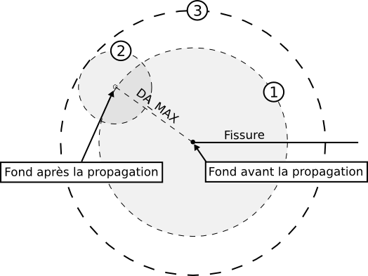
Figure 4.2-4 : selecting the nodes to be projected
We can look at the example given figure for a crack in 2D. The maximum progress of the crack is chosen by the user using the parameter DA_MAX of the PROPA_FISS operator. The position of the bottom of the crack after the propagation is therefore included in the circle whose center coincides with the position of the bottom before the propagation and whose radius is equal to the value of DA_MAX (circle 1 in the figure). The nodes used to calculate the local residue are included in the circle whose center coincides with the position of the background after the propagation and whose radius is equal to the value of the parameter RAYON of the PROPA_FISS operator (circle 2 in the figure). For the projection, it is therefore possible to select all the nodes included in the circle whose center coincides with the position of the background before the propagation and whose radius is equal to the addition of DA_MAX and RAYON (circle 3 in the figure).
Finally, it should be noted that the projection proposed above calculates the new value of the level-sets only for the nodes that have been projected. However, for the other X- FEM routines in Code_Aster to work properly, it is necessary that the physical mesh level-sets be defined for all nodes. To do this, you can simply preserve the value of the level-sets for all the nodes that are not affected by the projection. Each time, we can therefore take the physical mesh level-sets before the propagation and we can change the value of the level-sets only for the nodes affected by the projection. This solution is very easy to develop in code and is very fast. In addition, it ensures that the existing surface of the crack and the bottom of the crack are always correctly represented by the level-sets because the results of each projection are preserved behind the crack background. An example is shown in figure. On the left side of the figure we see the configuration of the level-sets before the update. The surface of the crack is shown in orange and the bottom is marked with a small orange. The configuration of the level-sets after the propagation (and the projection) is visible on the right. Only the level-sets at the nodes in circle 3 have been replaced by the new values calculated on the auxiliary grid. The new surface of the crack is shown in red and the new position of the bottom is represented by a small red. The position of the background before propagation is always marked by an orange dot. It can be seen that the surface of the crack that existed before the propagation is preserved by the projection (red line to the right of the orange point), as well as the continuity of the crack surface between the projection domain (circle 3) and the remaining part of the physical mesh (the red line is the continuation of the orange line). With the definition of the projection domain used, the level-sets around the position of the crack background before the propagation (orange point) are always affected by the projection and there is therefore no risk of false crack foundations being detected (\(\mathit{lsn}\mathrm{=}\mathit{lst}\mathrm{=}0\)) after the projection. It can also be noted that the level-sets are discontinuous for physical meshing but that this is not important. Indeed, the orthogonality and signed distance properties of the level-sets are guaranteed for all the nodes involved in the calculations on the physical mesh.
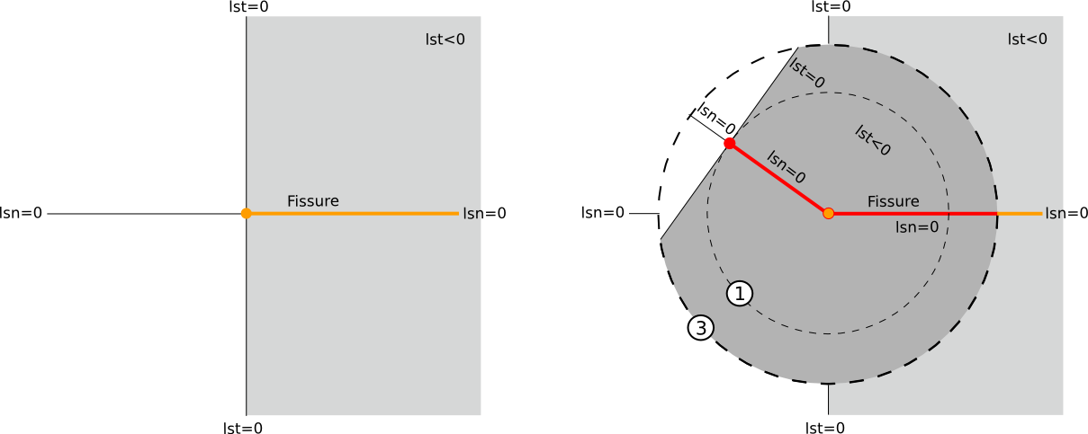
Figure 4.2-5 : configuration of level-sets on the physical mesh before (left) and after (right) propagation. The area where the tangent level-set is negative is t ei**nt in gray. The surface and the bottom of the crack are shown in orange before propagation and in red after it has spread.**
Note that the level-sets are updated on all the nodes of the auxiliary grid and that for this mesh their representation is correct everywhere. So for the auxiliary grid we do not have the discontinuities that we find on the physical mesh after the projection (figure), except in the case of using the location of the computing domain described in paragraph [§ 5], which does not represent a problem.
4.2.2. « Simplex » method#
The use of the auxiliary grid is not always convenient for the user, especially for complex structures. With this in mind, a method based on the same idea as the upwind method was developed. Still using a fast marching algorithm, we will simply modify the calculation at the element level and work directly on simplex elements [:ref:` 22 < 22 >`] (triangle, tetrahedron).
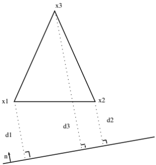
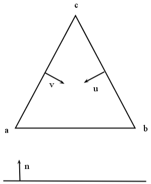
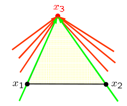
Figure 4.2-6: Simplex method on a triangle
To simplify things, let’s take the example of a 2D case. We consider a triangle mesh with \({x}_{1}\), \({x}_{2}\), and \({x}_{3}\), the coordinates of the three nodes of the triangle (see). Assuming the linear crack background piecewise, we can project each of the points onto this one. So \(n\) is the normal, unknown, and element-wise constant.
Keeping in mind that the three points project onto a normal line \(n\), we have \({d}_{1}\), \({d}_{2}\), and \({d}_{3}\) that represent the level-set values on each of the three nodes. Since \({d}_{1}\) and \({d}_{2}\) are known, we are therefore looking for a way to calculate \({d}_{3}\). The idea used is like writing the equation for the projection of a point on a line for \({x}_{1}\), \({x}_{2}\), and \({x}_{3}\). We have:
Or even:
So we have a system of two equations and three unknowns. To obtain a solution, we will put the system in vector form:
With:
\(V\) is invertible because the cells are non-degenerate, which allows the unknown \(n\) to be written in the following form:
Since \(n\) is a unit vector, we can eliminate this equation from our system by writing only \(1={n}^{t}n\). Using the expression (), we end up with a quadratic equation where \({d}_{3}\) is the solution:
We end up with two solutions for the quadratic equation. For a consistent solution, choose the largest root of the equation.
Choice of the solution to the quadratic equation
Solving the system () leads to two solutions:
These two solutions are valid, but for our problem, we choose to keep () because it is the only one that meets the condition of obtaining increasing level-set values \({d}_{3}>{d}_{2}\) or \({d}_{3}>{d}_{1}\).
We observe several possible configurations in our problem. Let’s look at all of them to be convinced of the choice of this solution.
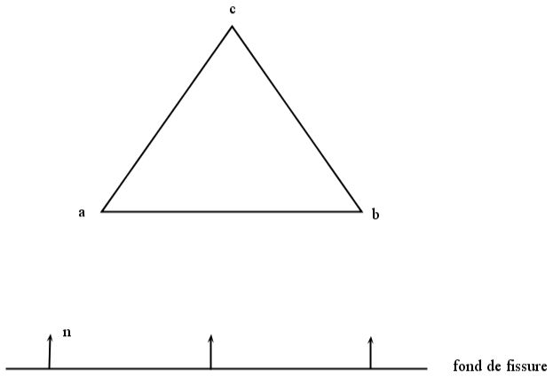
Figure 4.2-7: First configuration
In the first configuration (see figure ()), we know the value of the level-sets at points \(a\) and \(b\) and we look for the value at point \(c\). The \({x}_{1}\) solution of () gives a normal :math:`` and the solution in \({x}_{2}\) of () gives a normal \(\vec{{n}_{2}}(0;-1)\).
The solution () is therefore the one that gives the exact solution of the level-set value at point \(c\), and that respects the condition \(\mathit{ls}(c)>\mathit{ls}(b)\) or \(\mathit{ls}(c)>\mathit{ls}(a)\). The value obtained with solution () in this case gives \(\mathit{ls}(c)<\mathit{ls}(b)\) and \(\mathit{ls}(c)<\mathit{ls}(a)\).
The area of validity of the solution () for our problem can be identified. We look at the case where the quadratic equation has only one root (double root), see figure ().
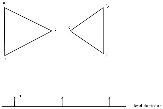
Figure 4.2-8: Second configuration
We see the two configurations of a triangle mesh that generate a double solution for the problem (discriminant equal to \(0\)). We can therefore identify the areas where the solution () and the solution () are valid in figure ().
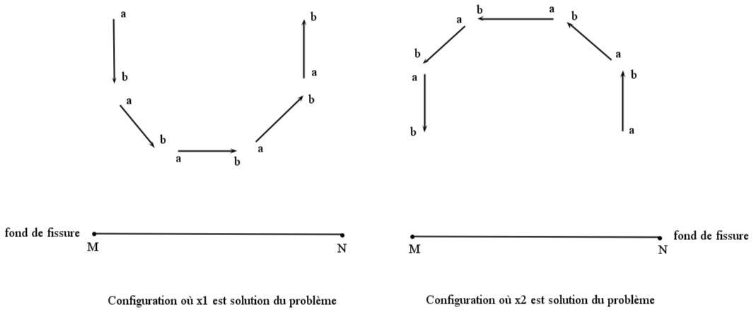
Figure 4.2-9: Third configuration
The solution () is accurate for our problem when \(\vec{\mathit{ab}}\cdot \vec{\mathit{MN}}\ge 0\), and the solution () when \(\vec{\mathit{ab}}\cdot \vec{\mathit{MN}}\le 0\).
The idea of the method being to start from the lowest level-set values, close to iso-zero, and to propagate these values, we can see that the solution () is the best suited. We therefore choose to take the largest root of the quadratic equation in our process of resetting the level-sets, regardless of the configuration. The strength of fast marching is to calculate the level-set value for the same node several times in different configurations around a node and to keep the best value. This therefore fixes the pathological cases where the solution () was taken when it was () who calculated the exact solution (i.e. there is at least one mesh containing the node in question for which the solution () is valid).
To ensure that the solution is monotonic and increasing, a criterion can be added to the choice of the solution.
Figure 4.2-10: Fourth configuration
Let \({d}_{1}\), \({d}_{2}\), and \({d}_{3}\) be the values of the level-set on any triangle mesh. So we want that if \({d}_{1}\) and \({d}_{2}\) increase then \({d}_{3}\) increases as well. The idea is to consider a level-set gradient:
As the solution is increasingly monotonic, we want \({({\nabla }_{d}{d}_{3})}_{i}>0,i\in ⟦1;2⟧\). By deriving the quadratic equation (), we have:
: label: eq-50
2 {d} _ {3} {nabla} _ {d} {d} {d} _ {3}mathrm {.} {I} ^ {t}mathit {QI} -2 {nabla} _ {d} {d} _ {3}mathrm {.} {I} ^ {t}mathit {Qd} -2 {d} _ {3}mathit {QI} +2mathit {Qd} =0
From where:
For \({({\nabla }_{d}{d}_{3})}_{i}>0\), you need to:
: label: eq-52
{begin {array} {c} {({mathit {QV}}} ^ {t} n}} ^ {t} n)} _ {i} >mathrm {0,} iin 1; 2\ {{{({mathit {QV}} ({mathit {QV}}}}} ^ {t} n}}} ^ {t} n)} _ {t} n)} _ {i} >mathrm {0,} iin 1; 2\ {{{({mathit {QV}}}}} ^ {t} n)} _ {t} n)} _ {i} <mathrm {0,} iin 1; 2end {array}; 2end
We saw earlier that if \({d}_{3}>{d}_{2}\) and \({d}_{3}>{d}_{1}\), we have \({({V}^{t}n)}_{i}<0\). Since \(Q\) is symmetric definite positive, the only possibility for \({({\nabla }_{d}{d}_{3})}_{i}>0\) is that \({({\mathit{QV}}^{t}n)}_{i}<\mathrm{0,}i\in ⟦1;2⟧\). In 2D, this means that \(\vec{n}\) must come from inside the triangle.
Proof
We have \({\mathit{QV}}^{t}V=I\) and we ask \({\mathit{QV}}^{t}=B=\left(\begin{array}{c}\vec{u}\\ \vec{v}\end{array}\right)\). So we have \(\mathit{BV}=I\iff \{\begin{array}{c}\vec{u}\cdot \vec{\mathit{ca}}=1\\ \vec{u}\cdot \vec{\mathit{cb}}=0\\ \vec{v}\cdot \vec{\mathit{ca}}=0\\ \vec{v}\cdot \vec{\mathit{cb}}=1\end{array}\)
To solve the problem, we ask \(\parallel \vec{u}\parallel =\frac{1}{\parallel \vec{\mathit{ca}}\parallel \mathrm{cos}(\alpha )}\) and \(\parallel \vec{v}\parallel =\frac{1}{\parallel \vec{\mathit{cb}}\parallel \mathrm{cos}(\beta )}\) where \(\mathrm{cos}(\alpha )\mathit{et}\mathrm{cos}(\beta )\ne 0\) .We want \({(\mathit{Bn})}_{i}<0\Rightarrow \{\begin{array}{c}\vec{u}\cdot \vec{n}<0\\ \vec{u}\cdot \vec{n}<0\end{array}\Rightarrow \vec{n}\) to come from inside the triangle.
4.2.2.1. Simplex method algorithm#
The path of the meshes in the structure remains similar to that of the upwind method. We select the node where the level-set reaches its minimum and we explore the triangles around this one to calculate the unknown values.
For each triangle in the mesh, we calculate the quadratic equation and keep the largest root
The propagation direction \(n={V}^{-t}(d-{d}_{3}I)\) is used to check a monotony criterion.
By replacing \(n\) in, we get:
This criterion means that \(n\) must come from within the triangle. In this way, the monotony of the solution is ensured.
If this condition is not met, the minimum value for one side of the triangle is taken.
Note: Generalization in 3D is very natural, the formulas being the same. The only difference comes when condition \({(Q(d-{d}_{3}I))}_{i}<\mathrm{0,}i\in ⟦\mathrm{1,3}⟧\) is no longer respected: we then calculate the smallest distance on each face of the tetrahedron and keep the smallest.
Unlike the upwind method, we no longer need the geometric method for edge points. The geometric method is used only to obtain the initialization values of the tangent level-set, always with the idea that the level-sets should remain orthogonal to each other.
4.3. Calculating level-sets near iso-zeros#
The methods presented above only give exact results if the iso-zeros in the level-sets actually pass through nodes. When the iso-zero passes between two nodes, it tends to be slightly deformed during the reset. An algorithm for calculating iso-zeros is therefore put in place. This geometrically calculates the distances signed on the nodes of the cells cut or tangented by the iso-zero of the level-set and sets the value calculated for the reset.
Regarding reorthogonalization, the values of \(\mathit{lst}\) located on the surface \((\mathit{lsn}\mathrm{=}0)\) must not be modified; we will therefore take advantage of the calculation algorithm of \(\mathit{lsn}\) to calculate the orthogonal lst values on the elements cut or tangented by \((\mathit{lsn}\mathrm{=}0)\) and freeze these values during the reorthogonalization phase. To do this, the value of \(\mathit{lst}\) is interpolated on the triangles \(\mathit{IJK}\) that can be formed with the intersection points \((\text{lsn}=0)\cap \text{arêtes}\). If for a \(M\) node, the orthogonal projection of \(M\) is inside \(\mathit{IJK}\), we interpolate the value of \(\text{lst}(M)\) as \(\mathit{lst}\) of the projected point. Otherwise, \(\text{lst}(M)\) is calculated as \(\mathit{lst}\) of the projected figure brought inside triangle \(\mathit{IJK}\) (Figure 4.3-1).
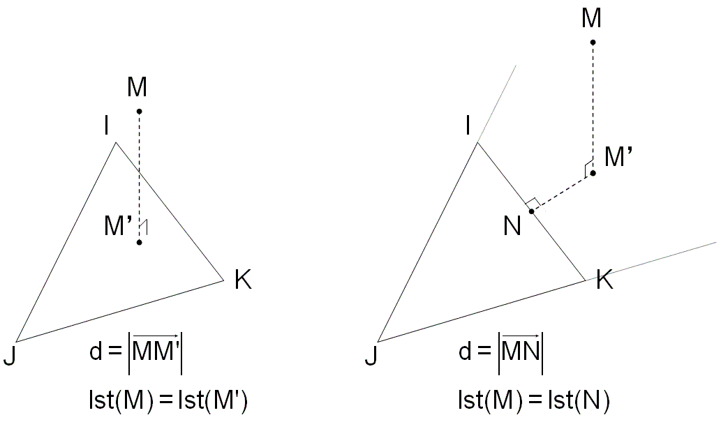
Figure 4.3-1 : Distance calculation and LST interpolation on elements cut by \(\mathit{lsn}\mathrm{=}0\) .
In 3D, the algorithm put in place after the propagation of \(\mathit{lsn}\) and before it was reset is as follows:
Loop on the stitches
If at least three knots of the stitch are on \(\mathit{lsn}\mathrm{=}0\), it is marked as a cut stitch
If the mesh has a \(\mathrm{[}\mathit{AB}\mathrm{]}\) edge such as \(\text{lsn}(A)\text{.}\text{lsn}(B)<0\), we identify the cut mesh
End of loop
Loop on the knots
If the knot belongs to a cut stitch, it will have to be calculated
End of loop
Loop on nodes \(P\) to be calculated
Loop on the cut stitches whose knot is at the top
Loop on the \(\mathrm{[}\mathit{AB}\mathrm{]}\) edges of the mesh
If \(\text{lsn}(A)\text{.}\text{lsn}(B)\le 0\), we interpolate the point \({I}_{\text{AB}}\):
\(\overrightarrow{{\text{AI}}_{\text{AB}}}=s\text{.}\overrightarrow{\text{AB}}\) with \(s=\frac{\mid \text{lsn}(A)\mid }{\mid \text{lsn}(A)\mid +\mid \text{lsn}(B)\mid }\)
and \(\text{lst}({I}_{\text{AB}})=\text{lst}(A)+s\text{.}(\text{lst}(B)-\text{lst}(A))\)
End of loop
Loop over all the \(\mathit{IJK}\) triangles that can be formed with the \({I}_{\text{AB}}\) dots
We calculate the projection \(M\) of \(P\) on the triangle \(\mathit{IJK}\)
We identify if the projected point \(M\) is inside the triangle
We store the distance \(d\mathrm{=}\mathit{PM}\)
We interpolate \(\text{lst}(M)\) linearly from \(\text{lst}(I)\), \(\text{lst}(J)\) and \(\text{lst}(K)\)
End of loop
End of loop
Among the calculated \(\mathit{PM}\) distances we are looking for the smallest distance with \(M\) within \(\mathit{IJK}\). If no projection inside \(\mathit{IJK}\) has been found, just take the smallest calculated distance and the corresponding \(\mathit{lst}\) value.
We store the corresponding \(d\) and \(\mathit{lst}\) values for node \(P\).
End of loop
We replace :math:`mathit{lsn}` and :math:`mathit{lst}` on the nodes to be calculated by the new stored values of*d*and*lst.
Nodes identified as « calculated nodes » have level-sets that are then frozen during the \(\mathit{lsn}\) reset and \(\mathit{lst}\) reorthogonalization phases.
The algorithm launched after the propagation and reorthogonalization phases of \(\mathit{lst}\) and before it was reset is the same, but it only calculates the \(\mathit{lst}\) distances, in the same way as \(\mathit{lsn}\) previously, without touching the values of \(\mathit{lsn}\).
The algorithm described above is valid only in 3D because in 2D you cannot form triangles. In fact, only two intersection points can be detected for each element.
To use the same algorithm in 2D as for the 3D case, the following solution can be used. A triangle is formed using the two intersection points (\(A\) and \(B\)) and a virtual point (\(C\)). This is chosen so that the triangle formed is in a plane orthogonal to the plane of the model (plane \(X\mathrm{-}Y\)). To avoid numerical problems, the coordinates of the virtual point (\(C\)) are calculated in the following way:
\(X,Y\) = coordinates of the midpoint of the edge connecting the two intersection points (\(A\) and \(B\)),
\(Z\) = distance between the two intersection points (\(A\) and \(B\)).