7. Mesh method for updating level-sets#
The most intuitive way to update level-set values at each crack propagation step is to use their signed distance property. This involves an explicit representation of the crack (crack lips and crack bottom) propagated in order to calculate the distances from the nodes to the crack. This method thus uses two distinct meshes (crack and structure) and only the crack mesh is modified during propagation. Updating the crack mesh at each propagation step consists in creating a new row of surface cells to represent the progress of the crack and a new row of line cells to represent the new background. Once this mesh is updated, the new level-sets are recalculated by direct calculation of the distance to the crack (orthogonal projection on the crack mesh).
7.1. Presentation of the method#
The crack is meshed in Code_Aster using the PROPA_FISS command. The input data is the value of the propagation vector on the crack front, determined from the stress intensity factors and the Paris law. The principle of the mesh method is to calculate the nodes of the new background from the propagation speeds and the nodes of the current background. It comes down to the following three steps:
Calculation by linear interpolation of the propagation vector at each node of the discretized crack front. The propagation vector is orthogonal to the crack front: the direction of propagation at a node corresponds to the average of the normal vectors of the two linear elements sharing this node. This step gives the position of each propagated point.
Addition of a node at each of these points, creation of a new surface (addition of linear elements for the new crack front and quadrangle elements for the new surface) and the process of meshing this created surface.
Specific treatment of edge knots which, depending on the case, can « leave » the structure. They are then moved across the borders of the structure.
For 2D models, the method is even simpler. Only one linear element needs to be added to each propagation step and no edge point correction is required.
7.2. Algorithm#
The algorithm set up for propagation by the mesh method is as follows (as described in (bib 20) and in the figure). At iteration \(i\):
Recovery of the crack mesh,
Recovery of the end points of the crack front,
Correction of the crack mesh:
We change the coordinates of the two end nodes of the crack front so that they correspond to the end points of the crack front
We change the coordinates of all the other nodes in the background so that they are evenly distributed between the two ends (number of nodes in the background \(\mathit{NbNf}\)).
Loop on the bottom knots: \(1⩽k⩽\mathit{NbNf}\)
Calculation of \(\Delta G(k)\) by linear interpolation,
Calculation of the bifurcation angle \(\beta\) from \({K}_{I}(k)\) and \({K}_{\mathit{II}}(k)\),
Calculation of the propagation vector by linear interpolation:
\(\Delta a(k)=C{\left(\Delta G(k)\right)}^{m/2}\) if \(C\) and \(m\) are filled in,
\(\Delta a(k)={\mathit{DA}}_{\mathit{MAX}}{\left(\Delta G(k)/{\mathit{max}}_{k}(\Delta G(k))\right)}^{m/2}\) if \({\mathit{DA}}_{\mathit{MAX}}\) and \(m\) are filled in,
Calculation of the position of the propagated of node \({N}_{k}\),
Addition of a new node.
end of loop
Loop between \(1\) and \(\mathit{NbNf}-1\)
addition of a new SEG2 stitch between each of the bottom knots and the next node,
addition of a QUA4 mesh between two successive nodes in the background to iteration \(i-1\) and their propagates,
in 2D: addition of a POI mesh for the background and SEG2 between the previous background and the new background.
End of loop,
Creation of meshes \(\mathit{FOND}\) (new background) and \(\mathit{LEVRE}\) (previous lip + new surface meshes),
Updating the mesh.
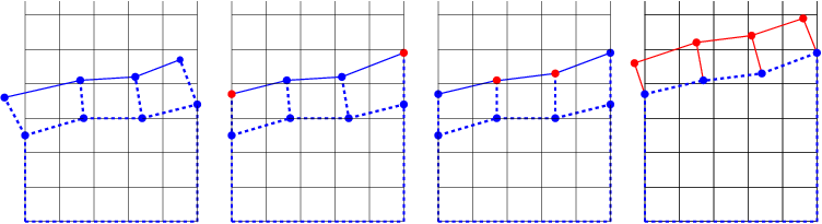
Figure 7.2-1 : a. mesh as input to the routine, b. step of correcting the edge points, c. step of equidistributing all the other nodes of the front, d. propagation of the discretized front and creation of the new meshes ( SEG2 and QUA4 ) .