7. Management of incompatibilities in contact processing#
The presence of contact and Dirichlet boundary conditions imposed on points on a common surface can generate redundancy problems leading to the failure of the calculation (in general, the tangent stiffness matrix becomes singular). In the following, we present some typical cases of redundancy that we identified, and the specific treatments proposed in [].
7.1. Redundancy between boundary conditions and contact and friction conditions#
7.1.1. example#
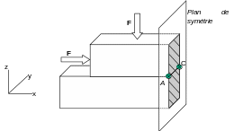
The most common case is a redundancy of the contact conditions with the boundary conditions. Take the example of a block in contact rubbing on a rigid plane (test case ssnv128, see): we model half of this block, at the end of which we apply the symmetry conditions: \({u}_{x}=0\). Loading is an imposed pressure \(F\) on the side and top faces. As has been said, the bottom face is in rubbing contact with its support. On segment \(\mathrm{[}\mathit{AC}\mathrm{]}\), we will have redundancy between the boundary condition and the sliding condition.
When we discretized the mixed variational formulation, we wrote that there was a coupling between the displacements and the friction semi-multipliers (matrices \(\left[{A}_{u}^{\Lambda }\right]\) and \(\left[{A}_{\Lambda }^{u}\right]\)), which means that the non-slip condition will give \({u}_{x}=0\), while this last condition is already imposed in the global system (the matrix \([B]\) of boundary conditions). So we impose the \({u}_{x}=0\) relationship twice. This situation results in a zero pivot error when inverting the tangent stiffness matrix.
|
Figure 13 : Plate in contact with friction on a rigid plane |
7.1.2. Choice of approximation space#
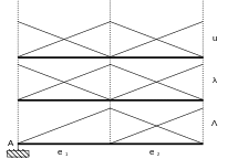
The solution adopted is to always give precedence to boundary conditions over adhesion-slip conditions. To do this, simply decouple the friction multipliers and the displacements for the component of the node concerned by the redundancy (to resume our example, we will decouple \({u}_{x}\) and \({\Lambda }_{x}\) to the nodes \(A\) and \(C\)). This is equivalent to changing the approximation space of the friction multiplier field by using a function that is equal to zero for the appropriate degree of freedom. This operation is illustrated in the figure in the 2D case where the redundancy condition is at point \(A\).
We take \({H}_{h}\) as the approximation space for the friction semi-multiplier \({\mu }_{h}\):
This space is in compliance with condition LBB. In practice, we simply put zeros in the appropriate locations of matrices \(\left[{A}_{e}^{\Lambda }\right]\) and \(\left[{A}_{\Lambda }^{e}\right]\) [bib3] _ .
The option SANS_GROUP_NO_FR/SANS_NOEUD_FR of Code_Aster allows you to remove the contribution to the friction matrix from a set of nodes, while maintaining the boundary and unilateral contact conditions in these nodes.
|
Figure 14 : Modifying approximation spaces for friction/boundary condition redundancy |
In 2D, one and only one direction of sliding exists. The removal of the adherence condition for problem points is therefore sufficient to eliminate any redundancy. It is done by decoupling the friction semi-multiplier associated with a connection of displacement unknowns.
In 3D, on the other hand, as slippage or adhesion occurs in the tangential plane, one may want to favor a particular sliding direction (for example perpendicular to a blockage). To do this, the user provides under the keyword DIRE_EXCL_FROT the direction to be excluded. This direction allows the construction of a local coordinate system that facilitates the decoupling of a single friction semi-multiplier. If no direction is provided then this amounts to not treating the friction on the nodes concerned (decoupling of the two multipliers).