6. Discretization of the mixed variational formulation#
This section describes the discretization of the problem defined by the variational formulations given p. 4. The variational formulations used have the following points in common:
Writing PTV for the balance of the structure, using a weak formulation of the equilibrium equation;
A vector field of unknowns: that of the primary variables representing either movements or speeds (in dynamics, in the case of the theta-diagram);
Geometry is represented by regular triangulation (classical polynomial finite elements);
An unknown scalar field representing the contact Lagrange multiplier \(\lambda\);
An unknown vector field representing the Lagrange friction semi-multiplier \(\Lambda\);
The Signorin contact model is applied weakly, with an enhanced Lagrangian formulation;
The Coulomb friction model is applied weakly, with an increased Lagrangian formulation;
Discontinuous sign fields for contact and friction have been introduced into the formulation.
In this chapter, we’ll introduce all the ingredients needed to make the discretized model and then, in the next chapter, we’ll look at how to solve the problem.
Important: from now on, we will note \(\lambda\) and not \({\lambda }_{n}\) the contact pressure to reduce the ratings. The friction pressure is always noted \(\Lambda\) .
6.1. Theoretical elements#
6.1.1. Paving the estate#
\({\Omega }^{i}\) domains are approached by polygonal \({\Omega }_{h}^{i}\) domains. Each domain \({\Omega }^{i}\) is associated with a family of \({T}_{{h}^{i}}\) triangulations with the parameter \({h}^{i}\), which is the mesh step of the domain \({\Omega }^{i}\). By noting \({K}_{j}^{i}\) the \({\mathit{NE}}^{i}\) elements of each triangulation, we can write:
: label: eq-219
{Omega} _ {h} ^ {i}mathrm {=}underset {jmathrm {=} 1} {overset {{mathit {NE}} ^ {i}} ^ {i}}} {mathrm {cup}}} {mathrm {cup}}}} {K} _ {j} ^ {i}}
For the discretization of the \({\Gamma }_{c}^{i}\) contact border, we are faced with an important first hypothesis. Indeed, this border can be discretized in two ways:
We take the geometric trace of the mesh of the underlying domain \({\Omega }^{i}\);
A new independent network is created, with its own discretization step.
In practice, the border mesh is almost always built on the first hypothesis, because otherwise this would involve meshing work that is difficult to implement, particularly in 3D. We will therefore always use the geometric trace of the mesh in domain \({\Omega }^{i}\) as a mesh for the contact border. The trace of \({T}_{{h}^{i}}\) forms a mesh \({T}_{{h}^{i}}^{\Gamma }\) of \({\Gamma }_{c}^{i}\). The discretized border \({\Gamma }_{c,h}^{i}\) is composed of \({\mathit{NE}}_{c}^{i}\) \({k}_{j}^{i}\) elements:
: label: eq-220
{Gamma} _ {c, h} ^ {i}mathrm {=}underset {jmathrm {=} 1} {overset {{mathit {NE}}} _ {c} ^ {i}} {c} ^ {i}}} {mathrm {cup}}} {k} _ {j} {NE}}} _ {mathit {NE}}} _ {mathit {NE}}} _ {mathit {NE}}} _ {c} ^ {i}} _ {c} ^ {i}}
6.1.2. Discrete approximation spaces#
The discrete version of space \({H}^{1}({\Omega }^{i})\), on domain \({\Omega }^{i}\), which will be noted \({H}_{h}^{i,q}\), is such that:
: label: eq-221
{H} _ {h} ^ {i, q}mathrm {=}mathrm {=}left{{u} ^ {u} ^ {i}mathrm {in} {(C ({stackrel {}} {omega} {omega}} {omega}} {omega}} {omega}} {omega}} {omega}}} ^ {i}))} ^ {i}))} ^ {i}))} ^ {i})} ^ {i})} ^ {i})} ^ {i})} ^ {i})} ^ {i})} ^ {i})} ^ {i}; {u} _ {K}} _ {j}} ^ {i}} ^ {i}} i}mathrm {in} {({P} _ {q} _ {q} ({K} _ {j} ^ {i}))} ^ {d}text {for} 1le jle {lele {mathit {NE}} {mathit {NE}}} ({K} _ {j} ^ {i} {i}right}
with \({\mathit{NE}}^{i}\) the number of elements coming from triangulation (), \(d\) the dimension of the problem, the dimension of the problem, \(C({\stackrel{ˉ}{\Omega }}^{i})\) the space of continuous functions on the adherence of \({\Omega }^{i}\) and \({P}_{q}({K}_{j}^{i})\) the space of polynomials with a degree less than or equal to \(q\) on the domain. The space containing the kinematically admissible functions has been designated by \({\mathit{CA}}^{i}\). The discrete version of this space, noted \({\mathit{CA}}_{h}^{i,q}\), is constructed as ():
: label: eq-222
{mathit {CA}} _ {h} ^ {i, q}mathrm {=}left{{u} ^ {i}mathrm {in} {(C ({stackrel {}} {} {omega}} {omega}} {omega}} {omega}}} {omega}}}} ^ {i}))} ^ {i})} ^ {i})} ^ {i})} ^ {i})} ^ {i})} ^ {i}; {u} _ {mid} {K} _ {j} ^ {i}) {i}} ^ {i}mathrm {in} {({P}} _ {q} ({K} _ {j} ^ {i}))} ^ {d}text {for} 1le jle {lele {mathit {NE}}} {mathit {NE}}}} {mathit {NE}}}} {mathit {NE}}}} {mathit {NE}}}} {mathit {NE}}}} ^ {i}} ^ {i}} ^ {i} _ {mathrm {mid} {gamma}} _ {Gamma} _ {u} {u} ^ {i}}}} ^ {i}mathrm {=} 0right}
We are going to write the discrete version of the space of the traces of functions on the border:
: label: eq-223
{mathit {CA}} _ {h} ^ {gamma, i} {gamma, i}mathrm {=}left{mathit {trace} ({u} ^ {i})text {on} {gamma}} _ {gamma}} _ {gamma}} _ {gamma}} _ {gamma}} _ {gamma}} _ {gamma}} _ {gamma}} _ {Gamma} _ {Gamma} _ {Gamma} _ {Gamma} _ {Gamma} _ {Gamma} _ {c}} _ {c}} _ {c} ^ {i}} _ {h} Gamma} _ {Gamma} _ {Gamma} _ {c}} _ {c} ^ {i}}}right}
From now on, we will forget the notation \(q\) to indicate the order of polynomials.
6.1.3. The Inf-Sup condition or condition LBB#
The mixed nature of the formulation imposes a dependence between the finite element spaces of the contact and friction multipliers and the finite element space of the displacements. This choice falls under the compatibility condition (or Inf-Sup condition or condition LBB of Ladyzenskaya-Babuska-Brezzi). A mechanical problem is generally reduced to solving a variational equation of the type:
: label: eq-224
text {Find} umathrm {in} Utext {such as}mathrm {forall} {u} ^ {text {*}}}mathrm {in} U mathrm {{}begin {array} {cc} {cc} a (u, {u}} ^ {text {*}})mathrm {=}mathrm {langle} l, {u}} ^ {text {*}} ^ {text {*}}}mathrm {*}}}mathrm {*}}}mathrm {*}}}mathrm {*}}}mathrm {*}}}mathrm {*}}}mathrm {*}}}mathrm {*}}}mathrm {*}}}mathrm {*}}}mathrm {*}}}mathrm {*}}}mathrm {*}}}mathrm {partial} Uend {array}
where \(U\) is a Hilbert space. It is often more convenient to rewrite this problem in a so-called mixed form, with two unknowns \(u\mathrm{\in }U\) and \(\lambda \mathrm{\in }M\):
: label: eq-225
text {Find} umathrm {in} Utext {and}text {and}lambdamathrm {in} Mtext {such as}mathrm {forall} {u}} ^ {text {*}} ^ {text {*}}}mathrm {in}}}mathrm {in} Utext {in} Mtext {in} Mtext {in} Mtext {such as}mathrm {forall} {u} ^ {text {*}} ^ {text {*}}}mathrm {*}}}mathrm {in} M {begin {array} {cc} a (u, {u}} ^ {text {*}}) +b ({u} ^ {text {*}}},lambda) =langle l, {u}} ^ {u} ^ {text {*}} ^ {text {*}} ^ {text {*}}} ^ {text {*}}},lambda) =langle g, {lambda} ^ {text {*}}}rangle &text {on}partial Uend {array}
where \(M\) is also a Hilbert space, dual \(U\) by the bilinear form \(b\). The problem is that the formulation given by () is not equivalent to the formulation given by (). Thus, in this very general framework, the equivalence of the two formulations, as well as a necessary and sufficient condition of existence and uniqueness (in addition, of course, to the classical hypotheses about the ellipticity and coercivity of the bilinear form \(a\)) of the solution of (), is given by the condition known as Ladyzenskaya, Babuska and Brezzka and Brezzuska of the bilinear form) of the solution of (), is given by the condition known as Ladyzenskaya, Babuska and Brezzka I* (LBB):
: label: eq-226
existsalphain >0,underset {{lambda} ^ {text {*}}}in M} {text {inf}}underset {{u} ^ {text {*}}}in U}in U} {text {lambda}}in U} {text {*}}}in U} {text {*}}}in U} {text {*}}}in U} {text {*}}}in U} {text {*}}}in U} {text {*}}}in U} {text {*}}}in U} {text {*}}}in U} {text {*}}}in U} {text {*}} text {*}})mid} {{parallel {lambda} ^ {text {*}}parallel} _ {M}\ mathrm {.} {parallel {u} ^ {text {*}}}parallel} _ {U}}gealpha >0
This condition indicates how to choose space \(M\), for the formulations to be equivalent. However, it must be admitted that from an operational point of view, we are not much more advanced, because this condition, which is very abstract, is also very technical to implement. Especially since this condition is expressed in the continuous framework and its passage in the discreet framework is not guaranteed! We will content ourselves with giving rules of application from the literature.
The application of condition LBB to our contact problem depends on the nature of the interfaces:
If the interface is left, obtaining an*Inf-Sup condition with a discontinuous discretization of the contact multipliers requires a very fine discretization of these multipliers;
If the interface is flat, space \({\text{CA}}_{h}^{\gamma ,i}\) of the traces of the movement fields on the contact interface as a space for discretizing the contact multiplier field meets condition LBB;
The continuous method uses the space of the traces of the displacement fields, knowing that stability (in the sense LBB) will not be guaranteed for non-plane interfaces.
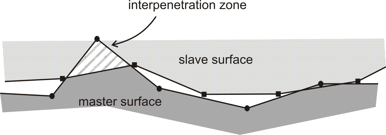
We take multiplier fields in space \({\text{CA}}_{h}^{\gamma ,i}\) throughout the contact interface [bib2] _ . For left surfaces (), this choice is convenient (since we discretize the multiplier field in the same way as the displacement field), but there is no proof of stability. In fact, the problem comes from the fact that the choice of one of the two surfaces as an integration surface constitutes a more or less rough approximation, as illustrated in. However, experience shows that this difficulty can be overcome by using approximation fields that are as smooth as possible (smoothing the normals, continuity of the multiplier fields). We will see later that compliance with the Inf-Sup condition is also strongly linked to the numerical quadrature scheme used to evaluate integrals.
|
Figure 6 : Incompatible left surfaces |
For the contact user in Code_Aster, this choice means that he may have convergence difficulties when the contact interfaces are left, the relative slippage is significant or the discretization difference is significant between the two surfaces.
6.1.4. Sign fields#
The choice of approximation spaces (of the polynomial finite element type) for the displacement field, the contact Lagrange multiplier field and the friction semi-multipliers field is not sufficient to build the discrete problem. There remains the case for sign fields (for contact, friction, speed field, etc.) which are naturally in infinite spaces. A collocation method is used to approximate these sign fields. We therefore choose a finite collection of points from the discretized contact surface \({\Gamma }_{c,h}^{i}\):
: label: eq-227
{({p} _ {j} ^ {i})}} _ {1le jle {n} _ {c} ^ {i}}mathrm {in} {Gamma} {Gamma} _ {c, h} _ {c, h} ^ {i}
A field with a \(S\) sign will therefore be approximated by \({S}_{h}\), which is the following discrete sum:
: label: eq-228
{S} _ {h}mathrm {=}mathrm {sum} _ {jmathrm {=} 1} ^ {{n} _ {c}} {omega}} {omega} _ {omega} _ {omega} _ {j} _ {j})
Careful! The number of collocation points \({n}_{c}^{i}\) is not necessarily the same as the number of points resulting from the finite element discretization of the touch/friction multipliers (which is based, as we recall, on the geometric trace of the discretized volume).
6.1.5. Digital integration#
To evaluate integrals numerically, it is necessary to choose an appropriate numerical quadrature scheme. This is based on the integration of discontinuous terms (sign fields) that « guide » the best schema to adopt. The question therefore moves to choosing the optimal collocation points to obtain precise contact efforts.
Compliance with the Inf-Sup condition was addressed in the context of the choice of functions for approximating the fields of contact and friction multipliers. Also in order to respect this condition, it was said that it was strongly linked to the precision of the digital integration that one is able to obtain. The phenomenon is understandable when we make the analogy with the methods of numerical sub-integration sometimes used to solve problems of numerical blockages due to an excessive richness of the approximation, by then « lowering » the degree of interpolation of fields by sub-integrating. The reasoning can therefore be easily overturned: if numerical integration « falses » (by enriching or impoverishing) the polynomial interpolation of multiplier fields, there is a risk of leaving the stability domain of condition LBB.
|
Figure 7 : Digital integration and compatibility |
This is the case, especially in case of incompatibility. Let us imagine that the elementary integration area on the slave surface covers several elements of the master surface. Since the non-zero support of test functions is a finite element, the fact of integrating numerically, by a Gauss quadrature, a non-polynomial function, but identically zero over a part of the integration area, is clearly not exact, because the quadrature is completely inappropriate (see). However, this is what we do when we try to integrate a functional field of a master element onto a much larger slave element (not compatible). By inverting the choice of surfaces, the result is clearly better (on the right), but there is still no guarantee of satisfactory integration. Next, we will describe the method adopted for*Code_Aster*, based on a subdivision of the element*which is only used for integration*. This method, which consists in refining the integration surface, limits the numerical integration error, and above all has the advantage of being extremely simple to implement.
Several ways have been explored to try to minimize these problems of incompatibilities between surfaces. The one selected in Code_Aster is to propose various digital integration schemes, which can be used according to needs. There are several types of schemes:
Digital integration at the nodes;
Digital integration at*Gauss points;
Numerical integration using the*Simpson method with 3, 5 or 9 integration points;
Integration by the*Newton-Cotes method with 4, 5 or 10 integration points;
Simpson integration makes it possible to improve the results in case of mesh incompatibility between the two contact surfaces, thanks to the subdivision of the integration elements that we have already mentioned above.
Newton-Cotes integration makes it possible to integrate polynomials of high order exactly (greater than three). It is very useful when the interpolation functions used on one of the two contact surfaces are of order greater than one (\(\mathit{P1}\mathrm{-}\mathit{P2}\), \(\mathit{P2}\mathrm{-}\mathit{P2}\)…). In addition, Newton-Cotes quadratures also allow (like Simpson’s) a subdivision of the integration element, and therefore apply in the event of mesh incompatibility.
However, one should be careful not to believe that the systematic use of a richer quadrature (Simpson, Newton-Cotes) is always a good choice. Firstly, because, in most cases, quadrature at the nodes is in practice sufficient (\(\mathit{P1}\mathrm{-}\mathit{P1}\) with sufficiently fine meshes). Second, because the richer a quadrature is (in terms of number of integration points), the greater the calculation volumes, and we will quickly realize that, for example, the use of the Newton-Cotes quadrature is quickly unacceptable. There is therefore no systematic a priory rule for choosing a quadrature, except for the few indications we have given: it is necessary to take into account the specificity of the model and the mechanical problem studied, and to make a compromise between the precision required for the solution and the necessary calculation time.
6.2. Contact elements#
After having discretized the mixed variational formulation and after having given the numerical integration schemes, all we have to do is set up finite elements for contact friction.
The idea of using finite elements is not an immediate step. For example, in discrete contact friction methods [R5.03.50], kinematic contact conditions are imposed without using finite elements and by intervening directly on the algebraic system to be solved. Such a strategy has the disadvantage of making programming and architecture completely dependent on the formulation, which prevents the contact from benefiting from improvements (architecture, performance) that would be achieved in the rest of the finite element code. On the other hand, we will see that developing finite contact and friction elements involves leaving the standard finite element diagram and that it is a suboptimal strategy from the point of view of performance.
To determine the stiffness matrix (and the second member) of the discretized system, the elementary terms of the finite elements must be calculated before assembling them. This elementary (classical) level is not sufficient for the treatment of our contact and friction problem. Several incompatibilities make the problem non-standard in the sense of finite elements.
6.2.1. Geometric incompatibility#
There is already a geometric incompatibility () between the discretizations of the two contact surfaces facing each other, a slave element, for example, being able to overlap several master elements.
|
Figure 8 : Geometric Incompatibility |
6.2.2. Incompatibility of the statutes#
The discontinuous nature of the contact/friction states leads to an incompatibility of the statuses (). Within the same contact element, several contact and friction states may coexist;

|
Figure 9 : Status Incompatibility |
This incompatibility is easily resolved because it is assumed that the sign field (thus indicating the contact and friction status) is discretized by collocation and that the collocation points have been chosen to be those of numerical integration. This means that the contact status is not carried by a contact element, but by a point of integration of a contact element.
6.2.3. Construction of contact elements#
It remains to build these contact elements. We are going to illustrate the principle on a 2D case.
|
Figure 10 : 2D example of pairing between two incompatible surfaces |
In the figure, we represent a 2D example of geometrically incompatible surfaces. The crosses represent integration points and here are the pairings and contact statuses:
Integration point |
Slave element |
Paired master element |
Status |
\(a\) |
|
|
Member |
\(b\) |
|
|
Slippery |
\(c\) |
|
|
Slippery |
\(d\) |
|
|
No contact |
\(e\) |
|
|
No contact |
\(f\) |
|
none |
No contact |
Table 6.2.3-1
There are therefore three contact elements that are represented in the figure. Each element is geometrically defined by the slave and master nodes. The status is represented by the collocation point, which acts as an integration point for each contact element.
|
Figure 11 : Creating the three contact elements |
We’ve put collocation points \((a,b,c,d)\) as Gauss points, but their location will of course depend on the integration diagram. Each contact element therefore represents a matrix or an elementary vector on the degrees of freedom carried by the slave nodes and by the master nodes. In 3D, the largest surface mesh is QUAD9 (quadrangle with nine knots), which is \(2\mathrm{\times }9\mathrm{\times }3\mathrm{=}54\) degrees of freedom for movement. In the case of contact with friction in 3D, three additional degrees of freedom per node are added to the slave surface: the Lagrange of the contact multiplier and the two Lagranges of the friction semi-multiplier, which gives an additional \(9\mathrm{\times }3\mathrm{=}27\) degrees of freedom. So in 3D, for the frictional contact element, the maximum size of the elementary matrix is \(81\) by \(81\) degrees of freedom.
In practice, the method is as follows:
Creation of the contact element on the master and slave nodes;
For each contact element, loop over the collocation points;
For each collocation point, calculation of the elementary matrix (or vector).
It is because of the last point that the creation of the finite element is suboptimal. In fact, we call it the calculation of the elementary matrix for each collocation point. However, for classical finite elements, the loop over the integration points is within the elementary calculation.
We therefore see that the use of a collocation scheme makes it possible to make different contact states coexist within the same element. However, there is still a compatibility problem between the EF approximation of the shape functions and the integration diagram. Take the example of a segment (figure).

|
Figure 12 : EF/collocation mismatch on a segment |
On this segment, the displacement is approximated by a linear function and it is equal to 0 at the left node and it is greater than zero at the right node. From the point of view of contact, this means that a point located in the middle of the segment will necessarily come off. However, the integration by collocation diagram does not necessarily indicate this state. There is a decoupling between the polynomial approximation of the displacements and the discretization by collocation of the sign fields. This means that the collocation method is perfect for areas with constant contact states on the element but is much less relevant if the contact condition varies. Such a situation generates oscillations in transition zones. These oscillations cannot be reduced by using more collocation points but by refining the mesh in this area.
Notes:
Since the contact and friction elements have no geometric meaning, they are not in conformity, without any impact on the quality of the result: they are infinitely flattened when there is contact, they can be very distorted and have « strange » connectivities in the case of connection between surfaces of different degrees;
The fact of using the integration diagram at the nodes does not make the contact elements more efficient in terms of their use, since the principle described above is generic for all integration schemes;
There is no procedure dedicated to perfectly compatible meshes. Two meshes chosen to be compatible will not give faster results than two incompatible meshes;
The fact of having to build late finite elements results in a refactoring of the global matrix at each Newton’s iteration, since the topology of the matrix will be modified.
6.3. Preparing for discretization#
6.3.1. Discretization in time#
The (pseudo-) -temporal discretization will be indicated by the clue \(k\). For example, the displacement \({u}_{k}\) at the current time step is written as the sum of the cumulative displacement \({u}_{k}^{\mathit{cum}}\) since the start of the Newton process of the current time step and the displacement increment of the current Newton iteration \(\Delta u\) that we are looking for:
: label: eq-229
{u} _ {k}mathrm {=} {u} _ {kmathrm {-} 1} + {u} _ {k} ^ {mathit {cum}} ^ {mathit {cum}}} +Delta u
This iterative writing is also valid for other nodal unknowns (Lagrange multiplier field):
: label: eq-230
{lambda} _ {k}mathrm {=} {lambda} _ {lambda} _ {kmathrm {-} 1} + {lambda} _ {k} ^ {mathit {cum}} ^ {mathit {cum}}} +deltalambda
And:
: label: eq-231
{Lambda} _ {k}mathrm {=} {Lambda} _ {kmathrm {-} 1} + {Lambda} _ {k} ^ {mathit {cum}} ^ {mathit {cum}}} +DeltaLambda
In Code_Aster, we made the choice to work in total quantity (and not incremental) for the Lagrange multipliers, so they are initialized to zero at the start of each time step and we therefore have:
And:
We’ll use a notation that separates known \({\stackrel{ˆ}{u}}_{k}\) and unknown \(\Delta u\) quantities at the current time step \(k\):
: label: eq-234
{u} _ {k}mathrm {=} {stackrel {} {u}} _ {k} +Delta u {stackrel {} {u}}} _ {k}mathrm {=} {stackrel {} {u}}} _ {k} +Deltastackrel {} {u}}} _ {k} +Deltastackrel {} {u}
For updated coordinates, like \(x\mathrm{=}p+u\):
: label: eq-235
{x} _ {k}mathrm {=} {stackrel {} {x}} _ {k} +Delta x {stackrel {} {x}}} _ {k}mathrm {=} {stackrel {} {x}}} _ {k} +Deltastackrel {} {x}}} _ {k} +Deltastackrel {} {x}
For the contact pressure field:
: label: eq-236
{lambda} _ {k}mathrm {=} {stackrel {} {lambda}} _ {k} +deltalambda
For the friction pressure field:
: label: eq-237
{Lambda} _ {k}mathrm {=} {stackrel {} {Lambda}} _ {k} +DeltaLambda
This notation remains valid for other quantities such as the increased contact multiplier:
: label: eq-238
{g} _ {n, k}mathrm {=} {stackrel {} {g}}} _ {n, k} + {delta g} _ {n}
And the increased friction semi-multiplier:
For the projection operator on the unit ball:
: label: eq-240
{stackrel {} {tau}}} _ {k}mathrm {=}frac {{stackrel {} {h}}} _ {tau, k}}} {{tau, k}}} {}} {, k}} {
6.3.2. Discretization of the local coordinate system#
We do not specify how the normals and tangents are interpolated, because everything will depend on the options specified in DEFI_CONTACT (activating smoothing for example). You just need to know that you use the same form functions as the description of geometry. We will write directly that the normal or the tangents are quantities expressed at the current point of integration:
: label: eq-241
nstackrel {text {Discretization}} {to} {to}left{{n} _ {h}right} {t} ^ {1}stackrel {text {Discretization}} {to}left{{t} _ {h} ^ {1} ^ {1}right} {t} ^ {2}stackrel {text {Discretization}} {to}left{{t} _ {h} ^ {2}right}
We will need to transform unknowns from the usual 3D space to the tangential plane. For this purpose, we use the rectangular matrix \(\left[{T}_{h}\right]\) such that:
: label: eq-242
left [{T} _ {h}right]mathrm {=}left [begin {array} {cc}left{{t} _ {h} ^ {1}right}right}} &left{{t}}} &left{{t}}right}left &left{{t}}right} &left{{t}}right} &left{{t}}right} &left{{t}}right} &left{{t}}right} &left{{t}}right
The discretization of the normal projection matrix is noted:
By developing the terms of normal \(n\) (discretized) and its three components in the global coordinate system \((x,y,z)\), we have:
: label: eq-244
left [{P} _ {h} ^ {n}right]mathrm {=}left [begin {array} {ccc} {n} _ {x} ^ {2} & {n} _ {x} {n} {n}} _ {n} _ {n} _ {x} {n} _ {x} {n} {n} {n} {n} {n} {n} {n} {n} {n} {n} {n} {n} _ {n} {n} {n} _ {n} {n} {n} _ {n} {n} {n} _ {n} {n} {n} _ {n} {n} {n} {n} _ {n} {n} {n} {n} _ {n} {n} {n} _ {y} ^ {2} & {n} _ {y} {n} _ {y} {n} _ {z} {n} _ {z} _ {z} & {n} _ {y} {n} _ {n} _ {n} _ {z} {n}} _ {n} {n} _ {z} {2}end {array}right]
Finally, the discretization of the tangent projection matrix is noted:
: label: eq-245
{underline {underline {P}}}} ^ {tau}stackrel {text {Discretization}} {to}left [{P} _ {h}} ^ {tau}right]
Be careful not to confuse \(\left[{P}_{h}^{\tau }\right]\) with the \(\left[{T}_{h}\right]\) () matrix on the tangential plane. \(\left[{P}_{h}^{\tau }\right]\) is worth:
: label: eq-246
left [{P} _ {h} ^ {tau}right]mathrm {=}left [begin {array} {ccc} 1mathrm {-} {n} _ {x} ^ {2} _ {x} ^ {2}} ^ {2}} &mathrm {-} ^ {2}} &mathrm {-} {n} {n} _ {x} {2} &mathrm {-} {n} {n} _ {x} {2} &mathrm {-} {n} {n} _ {x} {2}} &mathrm {-} {n} {n} _ {x} {2}} &mathrm {-} {n} {n} {n} _ {x} {} _ {z}\ mathrm {-} {n} _ {x} {n} _ {x} {n} _ {y} & 1mathrm {-} ^ {2} &mathrm {-} {n} {n} _ {n} _ {n} _ {y} {n} _ {z} {n} _ {z} {n} _ {z} {n} _ {z} &mathrm {-} {n} _ {y} {n} {n} _ {z} & 1mathrm {-} {n} _ {z} ^ {2}end {array} {n}end {array}right]
The matrices \(\left[{P}_{h}^{\tau }\right]\) and \(\left[{P}_{h}^{n}\right]\) are symmetric:
: label: eq-247
left [{P} _ {h} ^ {tau}right]mathrm {=} {left [{P} _ {h} ^ {tau}right]} ^ {tau}right]} ^ {T}
6.3.3. Discretization of solution fields#
Consider the vector field describing the geometry (node coordinates) on slave element \({p}^{e}\). This field has two or three components depending on the dimension of the space, we will note it in the following form:
Component \({p}_{x}^{e}\) is approximated by:
With \({\mathit{NN}}_{e}\) the number of nodes on the slave element, \({p}_{x,j}^{e}\) the J-th node value of the field following dimension \(x\) and \({N}_{j}^{e}\) the shape functions. By projecting on the basis of finite elements, the form functions being identical for the three dimensions of space:
: label: eq-250
{p} ^ {e}mathrm {=}left{begin {array} {c} {p} _ {x} ^ {e}\ {p} _ {y} ^ {e}\ {e}\ {p}\ {p} _ {p} _ {z} _ {z} ^ {e} _ {z} ^ {e} _ {z} ^ {e} _ {z} ^ {e} _ {z} ^ {e} _ {z} ^ {e} _ {z} ^ {e} _ {z} ^ {e} _ {z} ^ {e} _ {z} ^ {e} _ {z} ^ {e} _ {z} ^ {e} _ {z} ^ {e} _ {z} ^ {e} _ {z} ^ {=} 1} ^ {{mathit {NN}}} _ {e}}}left [begin {array} {ccc} {N} _ {j} ^ {e} & 0& 0\ 0& {N} _ {n} _ {j} {N} _ {e} _ {j} ^ {e} & 0\ 0& 0& {N} _ {j} ^ {e}\ end {array}\ right]0& {N} _ {array}right]left{begin {array} {c} {p} _ {x, j}} ^ {e} ^ {e}\ {p} _ {y, j} ^ {e}\ {p} _ {z, j} ^ {e}end {array}right}
We will write the nodal values \(\left\{{p}_{h}^{e}\right\}\) in more compact form:
: label: eq-251
{p} ^ {e}mathrm {=}left [{N} ^ {e}right]left{{p} _ {h} ^ {e} ^ {e}right}
In the same way for the master element:
: label: eq-252
{p} ^ {m}mathrm {=}left [{N} ^ {m}right]left{{p} _ {h} ^ {m} ^ {m}right}
For travel fields:
: label: eq-253
{u} ^ {e}mathrm {=}left [{N} ^ {e}right]left{{u} _ {h} ^ {e} ^ {e}right}
And for the current coordinate:
: label: eq-254
{x} ^ {e}mathrm {=}left [{N} ^ {e}right]left{{x} _ {h} ^ {e} ^ {e}right}
The contact multiplier field is scalar:
With \({\psi }_{j}\) the shape functions used for Lagrange multipliers. In more compact form, we will write:
: label: eq-256
lambdamathrm {=}mathrm {langle}psimathrm {langle}psimathrm {langle}left{h}right}mathrm {=}mathrm {langle}mathrm {langle}\ langle}psi {langle} {langle}psi {langle} {langle} {lambda} _ {h}rangle}left{\right}
The normal and the tangents must also be discretized. We start from the definition of the tangent coordinate system on the master cell, and we interpolate the normals and the tangents using the same shape functions. These discretized quantities will be noted \(\left\{{n}_{h}\right\}\), \(\left\{{t}_{h}^{1}\right\}\) and \(\left\{{t}_{h}^{2}\right\}\). When writing the various relationships, we assumed that the normal friction force density was an overall quantity, defined in the global coordinate system:
: label: eq-257
Lambdamathrm {=}left{begin {array} {c} {Lambda} _ {x}\ {Lambda} _ {y}\ {Lambda}\ {Lambda} _ {Lambda} _ {Lambda} _ {z}end {array}right}
The \({\Lambda }_{x}\) component on an edge element is written as follows:
: label: eq-258
{Lambda} _ {x}mathrm {=}mathrm {=}}mathrm {sum} _ {mathrm {=} 1} ^ {{mathit {NN}} _ {c}} _ {c}}} {c}}} {c}}} {Lambda}} {Lambda} _ {Lambda} _ {j}
With \({\mathit{NN}}_{c}\) the number of nodes on the edge element, \({\Lambda }_{x,j}\) the J-th nodal value of the \(x\) component of the frictional pressure field and \({\phi }_{j}\) the shape functions. In fact, as there is naturally a close relationship between contact and friction (that of the definition of the local coordinate system), the basic functions \({\psi }_{j}\) and \({\phi }_{j}\) are not independent, and the global friction Lagrange semi-multiplier \(\Lambda\) will be decomposed into two components (in 3D) into two components (in 3D) on the tangential plane defined at the point of contact by \(({t}^{1},{t}^{2})\):
: label: eq-259
Lambdamathrm {=}left{begin {array} {begin {array} {c} {Lambda} _ {Lambda} _ {Lambda} _ {z}{z}end {array}right}end {array}right} {right}}mathrm {=}} _ {sum} _ {jmathrm {=} 1} _ {z}z}end {array}rightright}}mathrm {=} 1} ^ {mathit {NN}} _ {e}}left [begin {array} {cc} {cc}left{{t} _ {h} ^ {1}right}} &left{{t} _ {h} ^ {2} ^ {2}right}right}right}end {array}right]text {}left [begin {array} {cc} {t} _ {h}} ^ {2} ^ {2}right}2}right}& {psi} _ {j}end {array}right]text {}right]text {}left{begin {array} {c} {Lambda} _ {j} ^ {1}\ {Lambda}\ {Lambda} _ {Lambda} _ {Lambda} _ {Lambda}\ {1}\ {Lambda}\ {1}\ {Lambda}\ {1}\ {Lambda}\Lambda}\ {1
Which we are going to rewrite in a more compact form:
: label: eq-260
Lambdamathrm {=}left [{T} _ {t} _ {h}right]left [psiright]left{{Lambda} _ {h}right}
If we consider the 3D case, the field of the friction semi-multiplier \(\Lambda\) is therefore of dimension three times the number of slave nodes. Its discrete version \(\left\{{\Lambda }_{h}\right\}\), projection on the tangential plane, has a dimension twice the number of slave nodes. We therefore only have three finite element bases that are a prima facie independent:
The base describing the geometry of the structure;
The base describing the primal field of unknowns (movement or speed);
The base describing the contact Lagrange multiplier and the projection of the friction semi-multiplier on the tangential plane at the contact point.
6.3.4. Digital integration#
The transformation of the continuous integral of a scalar quantity \(f\) into a discrete integral is written:
: label: eq-261
{mathrm {int}} _ {{omega} _ {h}}} fdomegamathrm {approx}mathrm {sum} _ {cmathrm {=} 1}} ^ {mathit {NP}}} ^ {mathit {NP}}} ^ {mathit {NP}}}} ^ {mathit {NP}}} f ({zeta} _ {c}) {omega} _ {c} _ {c}) {omega} _ {c} _ {c} _ {c}
With \(\mathit{NP}\) the number of integration points, \({\zeta }_{c}\) the parametric coordinate of the integration point on the slave cell, \({\omega }_{c}\) the integration weight of this point and \({J}_{c}\) the Jacobian of the transformation of the integration domain. This point is projected from the slave surface to the master surface by the matching application \({A}_{t}\). The evaluation on the master surface of the « paired » quantities noted \(\stackrel{ˉ}{f}\) is therefore simply written:
: label: eq-262
{mathrm {int}} _ {{omega} _ {h}}}stackrel {} {f} domegamathrm {approx}mathrm {sum} _ {cmathrm {=} 1} _ {cmathrm {=} 1}}}stackrel {} {f} ({A} _ {t}} _ {t} _ {t} ({zeta}) _ {c})) {omega} _ {c} {J} _ {c}
In the case of contact, it should be noted that each contact point is also a point of integration (method of discretizing the sign field by collocation). All continuous integrals will therefore be discretized by a numerical scheme combined with the method of collocation of sign fields.
6.3.5. Discretization of jumps#
The various quantities linked to the « jump » are functions of a quantity on the slave surface with its projection onto their master surface. First, let’s consider the projection of the jump onto the normal:
: label: eq-263
{mathrm {} umathrm {}}} _ {n}mathrm {=}mathrm {} umathrm {}mathrm {cdot} nmathrm {=} {=} (umathrm {-}}stackrel {} {u})mathrm {cdot} n
Recalling that \(u\) is a quantity defined on the slave surface and \(\stackrel{ˉ}{u}\) is its projection on the master surface. We will also need to develop tangential terms:
We recall the discretization defined on the unknown \(u\) by () using the shape functions defined at the current integration point \({\zeta }_{c}\) on the slave surface. The projection \(\stackrel{ˉ}{u}\) of this quantity onto the master surface will therefore use the integration point \({A}_{t}({\zeta }_{c})\) carried onto the master surface:
Which will be noted more compactly by:
: label: eq-266
umathrm {=}left [{N} ^ {e}right]left{{u} _ {h} ^ {e}right}
We finally have:
: label: eq-267
{mathrm {} umathrm {}}} _ {n}mathrm {=}mathrm {langle} {n} _ {h}mathrm {rangle} (left [{N} {}}} (left [{N} ^ {rangle}}} (left [{N}} ^ {rangle}} (left [{N}} ^ {rangle}} (left [{N}} ^ {rangle}} (left [{N}} ^ {rangle}} (left [{N}} ^ {rangle}} (left [{N} ^ {e}}) (left [{N} ^ {rangle}} (left [{N}} ^ {rangle}}) mathrm {-}left [{stackrel {} {N}}}} ^ {m}right]mathrm {{} {u} _ {h} ^ {m}mathrm {}})mathrm {}})mathrm {=}})mathrm {=}} (mathrm {=}} (mathrm {langle} {u} _ {h} ^ {e}mathrm {rangle}} {rangle} {left [{N} ^ {e}right]}} ^ {T}mathrm {-}mathrm {-}mathrm {langle} {u} _ {h} {m}mathrm {rangle} {rangle} {left} {left} {rangle} {rangle} {{}} {left} {rangle} {left} {left} {rangle} {left} {left} {left [{stackrel {} {N} {n}} {h}}}} ^ {T})left{{n} _ {h}right}
It’s a scalar. For the tangential jump:
: label: eq-268
{mathrm {} umathrm {}}} _ {tau}} _ {tau}mathrm {=}left [{P} ^ {tau}right] (left [{N} ^ {e}right]mathrm {e}right]mathrm {-}right]mathrm {-}right]mathrm {-}right]mathrm {-}right]mathrm {-}right]mathrm {-}right]mathrm {-}right]mathrm {-}right]mathrm {-}right]mathrm {-}right]mathrm {-}right]mathrm {-}\ stackrel {} {N}}} ^ {m}right]mathrm {{} {u} _ {h} ^ {m}}mathrm {}})
Now considering the normal jump of movement \({d}_{n}\):
So:
: label: eq-270
{d} _ {n}mathrm {=}mathrm {langle} {n}} _ {h}mathrm {rangle} (left [{N} ^ {e}right]mathrm {{}right]mathrm {}right]mathrm {}right]mathrm {stackrel]]mathrm {-}right]mathrm {stackrel}]mathrm {-}right]mathrm {stackrel] {} {N}} ^ {m}right]mathrm {{} {x} _ {h} ^ {m}mathrm {}})
Likewise:
: label: eq-271
{mathrm {} xmathrm {}}} _ {tau}} _ {tau}mathrm {=}left [{P} ^ {tau}right] (left [{N} ^ {e}right]mathrm {e}right]mathrm {-}right]mathrm {-}right]mathrm {-}right]mathrm {-}right]mathrm {-}right]mathrm {-}right]mathrm {-}right]mathrm {-}right]mathrm {-}right]mathrm {-}right]mathrm {-}right]mathrm {-}stackrel {} {N}}} ^ {m}right]mathrm {{} {x} _ {h} ^ {m}}mathrm {}})
From where:
: label: eq-272
{d} _ {tau}mathrm {=}left [{P}}left [{P} ^ {P} ^ {e}right]mathrm {{} {x} _ {h} {x} _ {h} ^ {e} _ {h} ^ {e}}left [{stackrel {} {x}} _ {x} _ {x} _ {h}} _ {h} ^ {e}} _ {h} ^ {e}} _ {h} ^ {e}} _ {h} ^ {e}} _ {h} ^ {e}} _ {h} ^ {e}}left [{stackrel {} {N} {x}} _ {x} _ {h}} _ {h} ^ {e}}right]mathrm {{} {x} _ {h} ^ {m}mathrm {}})
Quantities derived with respect to parametric coordinates:
: label: eq-273
frac {mathrm {partial}stackrel {} {x}} {mathrm {partial} {zeta} ^ {alpha}}mathrm {=}mathrm {partial}mathrm {sum}} _ {mathrm {sum}} _ {mathrm {sum}} _ {mathrm {sum}} _ {sum}} _ {mathrm {sum}} _ {sum}} _ {mathrm {sum}} _ {sum} _ {array} {sum} _ {sum} _ {array}} _ {m}}}left [begin {array} {sum}} _ {sum}} _ {array} {cc_ c}frac {mathrm {partial} {partial} {stackrel {} {N}}} _ {j} ^ {m}} {mathrm {partial} {zeta}} ^ {alpha}}} & 0& 0\ alpha}} & 0& 0\ 0&0&0&frac {mathrm {partial}} {stackrel {partial} {N}}} {zeta} ^ {alpha}}} & 0& 0\ alpha}} & 0& 0\ alpha}} & 0& 0\ 0&0&0&0&frac {mathrm {partial}} {N}}} _ {j} ^ {alpha}}} & 0& 0} {mathrm {partial} {zeta} {zeta}} ^ {alpha}} & 0\ 0&frac {mathrm {partial} {stackrel {} {N}}}} _ {zeta}} {zeta} {mathrm {partial}} {partial}} {partial} {partial} {partial} {partial} {partial} {partial} {partial} {partial} {partial} {partial} {partial} {partial} {partial} {partial} {partial} {partial} {partial} {partial} {partial} {partial} {partial} {partial} {partial} {partial} {partial} {partial} {begin {array} {c} {x} _ {j} _ {j} ^ {m} ^ {m} _ {j} ^ {m}\ {z} _ {j} ^ {m}end {array}right}
By noting \(\left[{\stackrel{ˉ}{B}}_{\alpha }^{m}\right]\) the matrix of derivatives of form functions with respect to the parametric coordinate \({\zeta }^{\alpha }\). That is:
6.3.6. Discretization of (semi) -multipliers#
Consider the increased contact multiplier \({g}_{n}\):
: label: eq-275
{g} _ {n}mathrm {=}lambdamathrm {-} {rho} _ {n} {d} _ {n} _ {n}
Its discretization gives:
: label: eq-276
{g} _ {n}mathrm {=}mathrm {langle}psimathrm {langle}left{{lambda} _ {h}right}right}mathrm {-} {-} {rho} _ {n}mathrm {rangle} (left [{N} ^ {e}right]mathrm {{} {x} _ {h} ^ {e}}mathrm {-}left [{stackrel {} {N} {N}}}} ^ {m} {x}}}left [{stackrel {} {N} {N} {N} {N} {N}}}}mathrm {}})
Now let’s consider the Friction Augmented Semi Multiplier \({h}_{\tau }\):
: label: eq-277
{h} _ {tau}mathrm {=}Lambda + {rho} _ {t} {v} _ {tau} _ {tau}
We consider incremental writing on the go (see § 5.2):
Discretizing the semi-multiplier gives:
: label: eq-279
{h} _ {tau}mathrm {=}left [Tright]left [Tright]left [psiright]left{{Lambda} _ {h}right}} + {stackrel {}} {stackrel {}} {rho}} {rho}}} _ {rho}}} _ {tau}right] _ {tau}right]mathrm {{} {u} _ {h} ^ {e} ^ {e}mathrm {}}mathrm {-}left [{stackrel {} {N}}}} ^ {m}\ right]mathrm {}right]mathrm {}right]mathrm {}right]mathrm {}right]mathrm {}right]mathrm {}right]mathrm {}right]mathrm {}right]mathrm {}right]mathrm {}right]mathrm {
6.3.7. Contact and friction statuses#
The contact sign field noted \({S}_{u}^{{g}_{n}}\) was defined by the following expression:
: label: eq-280
{S} _ {u} ^ {{g} _ {n}}mathrm {=}mathrm {=}mathrm {{}begin {array} {cc} 1&text {si} {c} 1&text {si} {g} {g} _ {g} _ {g} _ {n} _ {n} _ {n}mathrm {le} 0end {array} {cc} {c}begin {array} {cc} 1&text {si} {g} 0&text {si} {g} _ {g} _ {g} _ {n} _ {n}}mathrm {le} 0end {array} {cc} {c}begin {array} {cc} 1&text {si} {} _ {n} >0end {array}end {array}
This operator is the characteristic function of the increased contact multiplier \({g}_{n}\) on the convex \({\mathrm{ℝ}}^{\text{-}}\). The friction sign field noted \({S}_{f}^{{h}_{\tau }}\) has also been defined by the following expression:
: label: eq-281
{S} _ {f} ({h} _ {tau})mathrm {=}mathrm {=}mathrm {{}begin {array} {c} {c}begin {array} {cc} 1&text {si} {tau} _ {tau} _ {tau} _ {tau} _ {tau} _ {tau} _ {tau} _ {tau} _ {tau} _ {tau} _ {tau} _ {tau}\in} B (mathrm {0,} 1)end {array} {cc} 1&text {si} {i} {h} _ {h} _ {h} _ {h} _ {h} _ {h} _ {h} _ {tau} {cc} 0&text {else}end {array}end {array}end {array}
This operator is the characteristic function of the semi-multiplier increased by friction \({h}_{\tau }\) on the convex \(B(\mathrm{0,}1)\). Discretizing sign fields is trivial because collocation is used on these discontinuous fields (see § 6.1.4). The discretized value of a multiplier (contact or friction) is equal to its value at the point of integration. Since these operators are discontinuous, their linearization does not make sense. We therefore write the value of these fields directly at the current time \(k\) but just before the current Newton iteration:
: label: eq-282
{stackrel {} {S}}} _ {u, k} _ {u, k}} ^ {{g} _ {n}}mathrm {{}begin {array} {c}begin {array} {c}begin {array} {{array} {cc} {cc} 1&text {c}} {array} {cc} 1&text {c} {array} {cc} 1&text {c} {array} {cc} 1&text {c} {array} {cc} 1&text {c} {array} {cc} 1&text {c} {array} {cc} 1&text {c} {array} {cc} 1&text {c} {array} {cc} 1&text {si} {si} {{array}\ begin {array} {cc} 0&text {si} {stackrel {} {g}} _ {n, k} >0end {array}end {array}end {array}
6.3.8. Discretization of virtual quantities#
We will now consider writing discretized forms of virtual quantities. For \(\delta {d}_{n}\):
For \(\delta {d}_{\tau }\):
The variation of the semi-multiplier increased by friction is equal to:
6.4. Resulting discretized system#
We start again with the system (), which represents the balance of the system (PTV) in incremental form:
: label: eq-286
textrm {Find fields} ({u} _ {k} ^ {1}, {u}, {u} _ {k} _ {k} _ {1}, {lambda} _ {k})mathrm {in} {in} {text {CA}} {text {CA}}} {text {CA}} {k})mathrm {times}} {times} {k})mathrm {in} {in} {in} {text {CA}} {in} {in} {text {CA}} {in} {text {CA}} {in} {in} {text {CA}} {times}} {times} Hmathrm {times} H {begin {array} {cc}sum _ {i=1} {i=1} ^ {1}} ^ {i=1}} ^ {2}left ({W} _ {k}, {mathrm {delta}}, {mathrm {delta} W} W} ^ {k} W} W} _ {k}right) - {G} _ {text {int}, k} {i}left ({i}}k}left ({W} _ {k}, {mathrm {delta} W}} _ {k}right)right)right] - {G} _ {text {c}, k}left ({W} _ {k}, {mathrm {delta} W} W}} _ {delta} W} W}} _ {k} W} _ {k} W} _ {k} W} _ {k} W} _ {k} W} _ {k} W} _ {k} W} _ {k}, {right) - {G} _ {k}, {mathrm {delta} W} _ {k}right) =0& (a)\ {stackrel {~} {G}}} _ {text {c}, k}left ({W} _ {k}}, {k} _ {k}right) =0& (b)\ {stackrel {~} {k} {K}} {G}, {G}} _ {text {f}, k}left ({W} _ {k}, {mathrm {delta} W} _ {k}right) =0& (c)end {array} mathrm {forall} {delta W} _ {k}mathrm {in} {text {CA}} ^ {1}mathrm {times} {text {CA}} {text {CA}}}} ^ {2}mathrm {times} Hmathrm {times} Hmathrm {times} H
After discretization, we obtain the following linearized system:
: label: eq-287
{begin {array} {cc}sum _ {i=1} {i=1} ^ {2}left [{G} _ {text {int}, k} ^ {i} - {G} _ {text {ext}, k}, k}}} ^ {i}1} ^ {i}right] - {G} _ {text {f}, k}, k}, k} =0&right] - {G} _ {text {f}, k}, k}, k} = 0&right stackrel {text {Discretization}} {to} {to}left{{L}left{stackrel {~} {G}}} _ {text {c}, k} =0&stackrel {text {c}, k} =0&stackrel {text {L}, k}, k} =0&stackrel {text {c}, k} =0&stackrel {text {c}, k} =0&stackrel {text {c}, k} =0&stackrel {text {c}, k} =0&stackrel {text {c}, k} =0&stackrel {text {c}, k}, k} =0&0\ {stackrel {~} {G}}}} _ {text {f}, k} =0&stackrel {text {Discretization}} {to}left{{L}left{{L} _ {L} _ {f, k} _ {f, k}right} =0end {array} mathrm {forall} {delta W} _ {k}mathrm {in} {text {CA}} ^ {1}mathrm {times} {text {CA}} {text {CA}}}} ^ {2}mathrm {times} Hmathrm {times} Hmathrm {times} H
This system is linearized (see § 5.4):
: label: eq-288
left{begin {array} {c} {L} _ {u, k} _ {u, k}\ {L} _ {f, k}end {array}right}right}mathrm {approx}}}mathrm {approx}}\ approx}\}{L}\ {L}leftleft{begin {array} {c, k} {-} 1}\ {L} _ {c, kmathrm {-} 1}\ {L} _ {f, kmathrm {-} 1}end {array}right} +left [begin {array} {ccc} {J} {J} {J} {J} {J} {J} {J} {cu} {J} {J} {cu} {J} {J} {J} {J} {J} {J} {J} {J} {J} {J} {J} {J} {J} {J} {J} {J} {J} {J} {J} {J} {J} {J} {J} {J} {J} {J} {J} {J} {J} {J} {J} {J} {J} {J} {C} & {J} _ {cf}\ {J} _ {fu} _ {fu} & {J} _ {fc} & {J} _ {ff}end {array}right]left{begin {array} {c} {c}\ Delta {u} {c}\ Delta {array} {c}\ Delta {array} {c} {c}\ Delta {array} {c}\ Delta {array} {c}\ Delta {array} {c}\ Delta {array} {c}\ Delta {array} {c}\ Delta {array} {c}\ Delta {u} ^ {i}\ i}\ Delta {lambda} _ {n}\ DeltaLambdaend {array} {c} {c}\ m {=}left{begin {array} {c} {c} {L} {L} _ {u, kmathrm {-} 1}\ {L} _ {c, kmathrm {-} 1}\ {L} 1}\ {L} _ {c, kmathrm {-}} _ {f, kmathrm {-} 1}end {array}right}} _ {c, kmathrm {-} 1}end {array}right}} +left [begin {array} {-} 1}\ begin {array} {-} 1}end {array}right}} +left [begin {array} {-} 1}c} Jend {array}right]right]left{{Delta W} _ {k}right} mathrm {forall}delta Wmathrm {in} {in} {text {CA}} ^ {1}mathrm {times} {text {CA}}} ^ {2}mathrm {times}}mathrm {times} Hmathrm {times} H
After linearization, we therefore end up with a system of the following form:
With the vector of nodal unknowns (real or virtual) \(\mathrm{\langle }\delta W\mathrm{\rangle }\):
: label: eq-290
⟶mathrm {delta} W●=⟶begin {array} {cccc}mathrm {delta} {u} ^ {e} &mathrm {delta} {u} {u} ^ {m} &mathrm {delta} &mathrm {delta}mathrm {delta}mathrm {delta} {u} {u} ^ {m}} &mathrm {delta} {u} ^ {m} &mathrm {delta} {u} ^ {m} &mathrm {delta} {u} ^ {m} &mathrm {delta} {u} ^ {m} &mathrm {delta} {u} ^ {m} &mathrm {delta} {
The \([K]\) matrix:
: label: eq-291
left [Kright]mathrm {=}left [begin {array} {cccc}left [{K}} _ {mathit {ee}}} ^ {t}right] +left [{K}} _ {mathit {K}} _ {mathit {ee}}right] +left [{K}} _ {right] +left [{K}} _ {right] +left [{K}} _ {right] +left [{K}} _ {mathit {ec}}right] &left [{K} _ {mathit {K}} _ {mathit {ef}}right]\ left [{K} _ {mathit {me}}right] &left [{K}}right] &left [{K} _ {mathit {mc}}right] &left [{K}] &left [{K}} _ {mathit {mc}} _ {mathit {ce}}right] &left [{K}}] &right] &left [{K}}right] &left [{cc}}right] &left [{K} _ {mathit {cf}}right]\ right]\left [{K} _ {mathit {fe}}right] &left [{K}} _ {mathit {fm}}right] & left [{K} _ {mathit {fc}}}right] &left [{K} _ {mathit {ff}}right]end {array}right]
Vector \(\left\{L\right\}\):
: label: eq-292
left{Lright} =left{begin {array} {c} {array} {c} {L} _ {text {int}} ^ {e} + {c} ^ {e} + {L} _ {L} _ {f} _ {f} _ {f} ^ {e} _ {f} ^ {e} _ {f} _ {f} ^ {e} _ {f} _ {f} ^ {e} _ {f} _ {f} ^ {e} _ {f} ^ {e} _ {f} ^ {e} _ {f} ^ {e} _ {f} ^ {e} _ {f} ^ {e} _ {f} ^ {e} _ {f} ^ {e} _ {f} ^ {e} _ {f} ^ {e} {f} ^ {m}\ {stackrel {~} {L}}} _ {c} ^ {c}\ {stackrel {~} {L}}} _ {f} ^ {f}end {array}right}
The matrices \(\left[{K}_{\mathit{ee}}^{t}\right]\) and \(\left[{K}_{\mathit{mm}}^{t}\right]\) are the tangent matrices coming from the linearization of internal forces (discretization of Jacobian matrices \({J}_{uu}^{u}\), see p. 11.1.1). The other matrices come from the linearization of contact and friction terms (see § 5.4). The system to be solved will therefore be:
: label: eq-293
left [Kright]left{Delta Wright}mathrm {=}mathrm {-}left{Lright}
In the expressions developed, we will always consider the case of generalized Newton, based on the « incremental-iterative » discretization specified in § 6.3.1. The discretized quantities will be written in a single integration point with coordinate \({\zeta }_{c}\), in such a way that we will introduce the integration weight \({\omega }_{c}\) of this point and the Jacobian \({J}_{c}\) of the transformation of the integration domain:
: label: eq-294
{mathrm {int}} _ {{omega} _ {h}} _ {h}} fdomegastackrel {text {discretization}} {to} f ({zeta}} _ {c})omega (c) J
Important note: It should be noted that with the notations above it is actually \(\mathrm{-}\left[L\right]\) that we find to the right of the equal sign. However, as the touch-friction forces are added in the code to the internal forces which are themselves subtracted from the second member, there is no need to take this change in sign into account. The expressions that are written in the elementary terms of the code are therefore very identical to those presented.
The expression for the second member vector is found in the appendix to p. 69 and that of the matrix tangent to p. 72.