8. Cycling during the Newton process#
8.1. Problem#
The use of a Newton algorithm on non-differentiable quantities sometimes causes numerical cycling phenomena to appear. Rigorously, we can use Newton’s algorithm on quantities that are almost differentiable (in the classical sense), in this case, we will speak of B-differentiability [], that is to say that the points of non-differentiability belong to a zero measurement space. In practice, with the numerical approximations introduced by discretization and the transition to floating point algebra, it is « very unlikely » that we will encounter these points of non-differentiability, but cycling problems are not excluded, especially in the case where contact/friction couples with other non-linearities.
A cycle corresponds to the passage of a point of non-differentiability during the Newton process (i.e. from one Newton’s iteration to the next).
In [], there are three types (see figure):
The cycle on contact status: a point in the mesh changes alternately from a contact case to a non-contact case;
Cycling on the status of friction: a point in the mesh changes alternately from a case of sliding to a case of adhesion;
Cycling on the sliding threshold: a point in the mesh passes alternately from a forward sliding case to a backward sliding case;
From a more heuristic point of view, it is also shown that second-order cycles often cause non-convergence.
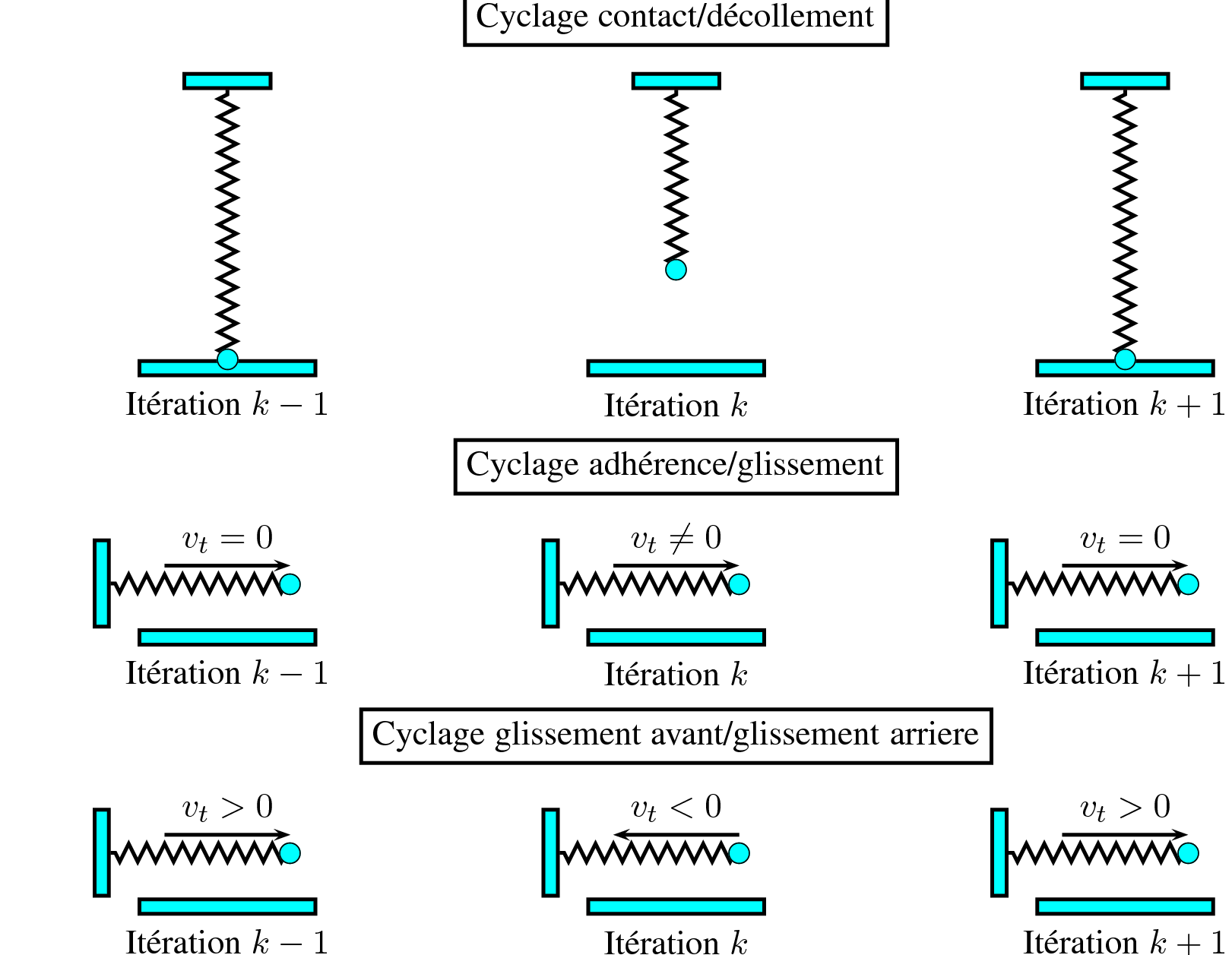
Figure 15: The different touch/friction cycles
8.2. Detection#
The three types of cycles are automatically detected.
8.3. Treatment#
8.3.1. Automatic cycling processing#
There is the possibility of automatically processing cycles such as touch/detachment, adhesion/sliding and sliding forward/backsliding (keyword ADAPTATION in DEFI_CONTACT).
For the keyword ADAPTATION =” CYCLAGE “, a generalized Jacobian base is built over two successive iterations: this base is used to modify the current contact and friction matrices. This manipulation is used for contact/detachment cycling. The cases of cycling forward/backsliding are treated so that the point is taken adherent as soon as the norm of its sliding is almost zero. In the case where the user requests a cycling-type treatment, the non-convergent points are automatically switched to penalization with an automatic control of the penalty coefficient (if the initial algorithm was an increased Lagrangian). The variational formulation in ALGO_CONT =” STANDARD “is thus modified. Indeed, in the expression of the original variational formulation. By noting, \({G}_{\text{c},k}^{\mathit{STD}}\) the weak contact force linked ALGO_CONT =” STANDARD “for all the points that do not cause problems, \({G}_{\text{c},k}^{\mathit{PENA}}\) for the points that have tipped, we have:
: label: eq-296
{begin {array} {cc}sum _ {i=1} {i=1} ^ {2}left [{G} _ {text {int}, k} ^ {i} - {G} _ {text {ext}, k} {k}, k} _ {text {ext}, k} _ {text {STD}} _ {text {}} _ {text {}} _ {text {}} _ {text}} c}, k} - {G} _ {text {f}, k} =0&stackrel {text {Discretization}} {to}left{{L} _ {u, k}right}right}right}}} =0\ {stackrel {~} {G}}} _ {text {c}, k} ^ {mathit {STD}}rightright}} =0stackrel {~} {G}}} _ {text {c}, k} ^ {mathit {}}rightright}} =0&stackrel {~} {G}}} ackrel {text {Discretization}} {to}left{{L}left{{L}} _ {c, k} ^ {mathit {STD}}right}} =0\ {stackrel {~} {G} {G}}}} {stackrel {~} {G}}}}} = 0\ stackrel {~} {G}}}} _ {text {G}}}} _ {text {G}}}} _ {text {G}}} _ {text {C}, k} ^ {mathit {PENA}} =0&stackrel {text {G} {G}}} {G}}} Discretization}} {to}left{{L} _ {c, k} _ {c, k} _ {c, k} _ {{L}}} _ {text {f}} _ {text {f}, k} _ {text {f}, k} _ {text}, k} _ {text {L}}} _ {text {f, f}, k} = 0&stackrel {text {f}, k} =0&stackrel {text {f}, k} =0&stackrel {text {f}, k} =0&stackrel {text {f}, k} =0&stackrel {text {f}, k} =0&stackrel {text {f} mathit {PENA}}right}} =0end {array} PENA
Finally, in cycling mode, to reinforce robustness, we do not wait for Newton’s convergence, which ensures that the pressures and the games are well within the cone of the admissible values \({\mathrm{ℝ}}^{-}\).
For the keyword ADAPTATION =” ADAPT_COEF “, there are two cases:
In increased Lagrangian (ALGO_CONT =” STANDARD “and ALGO_FROT =”” and =” STANDARD “), we will modify the increase coefficient to « break » the cycle between adherent status and sliding status at the same integration point. This modification of the coefficient is safe because it does not change the results, but just the speed of convergence. This mode is used to manage stick/slippery cycling. For this purpose, the following algorithm is used:
For a given coefficient of increase, we calculate the adherent/sliding status at the previous cycle and at the current cycle of the point detected as « cyclic »: are we close to the point of discontinuity (tolerance fixed at 5%)?
If yes, we modify the increase coefficient iteratively to get out of this critical zone while not approaching it on the other side;
If no, nothing is changed;
The adapted coefficient is propagated to the other points according to a specific algorithm (see § 8.3.2);
In stabilized Lagrangian (ALGO_CONT =” PENALISATION “), we will modify the regularization coefficients in penalization to automatically detect the cases of singular matrices and automatically process the maximum penetration calculated during the iterations: see § 8.3.3.
Notes on adherent/slippery cycling:
Because of the scaling of the Lagrangian friction projection (see § 3.2.4), the tolerance given (here 5% on either side of the point of discontinuity) does not depend on the units of the problem;
The cycling detection procedure showed a point that varies between the sliding status and the adherent status. The strategy adopted here consists in considering cases where one of the statuses is close to the point of discontinuity. If this is not the case (cycling between two areas far from the discontinuity or between two areas close to the discontinuity), the algorithm does nothing.
The algorithm for adapting the coefficient of increase is a simple loop that, at first, increases the coefficient of increase by multiplying it by two, and if we fail, starts again in the other direction by dividing the coefficient by two. The coefficient is chosen in the interval \(\mathrm{[}{10}^{\mathrm{-}8}{\mathrm{,10}}^{+8}\mathrm{]}\).
8.3.2. Algorithm for propagating the coefficient of increase in adherent/sliding cases#
The previous algorithm is only effective if a procedure is implemented that will propagate (or not) the optimal coefficient found on a cyclic point. In fact, in practice, such an optimal coefficient is very likely to be optimal for other points as well. This method thus makes it possible to anticipate the risks of cycling of points that are not yet in contact and makes the algorithm much more efficient.
To do this, during the coefficient adaptation procedure (§ 8.3.1 algorithm), the maximum and minimum values found over the entire contact zone are stored and the following algorithm is applied:
Loop on contact points
With the maximum coefficient on the contact zone, we evaluate on all points whether or not we are close to the point of discontinuity, we then have four situations:
This new coefficient does not change the situation of the point on the friction graph with respect to the old coefficient → we propagate the new coefficient;
This coefficient changes the situation of the point on the friction graph but the old situation was far from discontinuity→ the new coefficient is not propagated;
This coefficient changes the situation of the point on the friction graph, the old situation was close to the discontinuity and the new position moves away from the discontinuity→ we propagate the new coefficient;
This coefficient changes the situation of the point on the friction graph, the old situation was close to discontinuity and the new position changes status (crossing the discontinuity) → the new coefficient is not propagated;
With the minimum coefficient on the contact zone, we evaluate on all points whether or not we are close to the point of discontinuity, we evaluate the same situations as in the previous case;
End of the loop at the points of contact
8.3.3. Algorithm for initializing the penalty coefficient#
We will detail whether the use of the keyword ADAPTATION =” ADAPT_COEF “in the case of penalized contact. In some calculations using the contact penalty method, the matrix is singular from the first iteration of the first time step. This singularity is due to a poor choice of the initial penalty coefficients. To numerically detect this situation and treat it, we rely on the matrix assembled before the first factorization. In fact, we note that this situation occurs if the largest value on the diagonal (except for the Lagrange terms due to boundary conditions) is very far from the smallest value on this same diagonal.
The profile of the matrix assembled by looking at the diagonal is:
: label: eq-297
K=left (begin {array} {ccc}}stackrel {~} {K} &mathrm {..} & {B} _ {mathit {lagr}}\ mathrm {..}} & {K}} & {K} _ {K} _ {K} _ {K} _ {mathit {lagr}} &mathrm {pena}}} &mathrm {..}}{B} _ {mathit {lagr}}} &mathrm {..}mathrm {..} &mathrm {..} end {array}right)
With \(\stackrel{~}{K}\) the overall stiffness matrix reduced to diagonal terms without contact terms and \({K}_{\mathit{pena}}\) the contact penalty matrix such as:
: label: eq-298
{K} _ {mathit {pena}}} = {left (begin {array} {begin {array} {cc} {K} _ {11}} = {r} _ {n} {n} {int} _ {int} _ {int} _ {mathrm {int}} _ {int} _ {n} {int} _ {n} {int} _ {int} _ {n} {int} _ {int} _ {int} _ {int} _ {int} _ {int} _ {int} _ {int} _ {int} _ {int} _ {int} _ {int} _ {int} _ {int} _ {int} _ {int} _ {int} _ {{delta} {g} _ {n} (u) dmathrm {Gamma} &mathrm {..}\ mathrm {..} & {K} _ {{mathit {pena}}} _ {22}}} _ {22}}} _ {22}}} =frac {1} {{r}} _ {c}}} {g} _ {n} (u)mathrm {delta} {g} {g} _ {n} (u) dmathrm {Gamma}end {array}right)}} _ {mathit {ii}}
The terms of friction are deliberately omitted for the sake of simplicity. In this last expression, we recall that:
\({S}_{c}\) refers to contact status;
\({g}_{n}\) refers to the current contact gap;
\(\mathrm{\delta }{g}_{n}\) refers to the virtual contact gap;
The initialization algorithm currently treats two scenarios:
After assembling the \(K\) matrix, we calculate \({r}_{\mathit{min}}=\mathit{min}(\stackrel{~}{K}\cup {K}_{\mathit{pena}})\) and \({r}_{\mathit{max}}=\mathit{max}(\stackrel{~}{K}\cup {K}_{\mathit{pena}})\)
First scenario: :math: {r} _ {mathit {max}}} is very small but not zero and:math: left| (mathrm {log} ({r} _ {mathit {max}}) {mathit {max}}))right|/left| (mathrm {log} ({r}}) ({mathit {min}}))right|/left| (mathrm {log} ({r}}) ({r}} _ {r} _ {r} _ {r} _ {r} _ {r} _ {mathit {min}}) {mathit {max}}))right|}) |<4.
This case corresponds to the case most often encountered when a singular matrix is detected. It reflects two hypotheses observed in practice.
The first hypothesis is that we are in the presence of non-soft materials (significant overall structural stiffness so :math:`{r}_{mathit{min}}` very small comes from contact) and* that there is at least one point in contact initially ** (\({K}_{{\mathit{pena}}_{11}}\ne 0\)). If \({r}_{n}\) was chosen too big (ex: \({r}_{n}\gg E\) Young’s modulus of the hard body) then either \({K}_{{\mathit{pena}}_{22}}\) is zero or \({K}_{{\mathit{pena}}_{11}}\) is much greater than \(\mathit{max}(\stackrel{~}{K})\): you have to reduce \({r}_{n}\). A value less than \({r}_{\mathit{max}}\) is sufficient to properly initialize the penalty coefficient. Otherwise, if \({r}_{n}\) was chosen too small then either \({K}_{{\mathit{pena}}_{11}}\) is zero or \({K}_{{\mathit{pena}}_{22}}\) is much greater than \(\mathit{max}(\stackrel{~}{K})\): you have to increase \({r}_{n}\). A value less than \({r}_{\mathit{max}}\) is sufficient to properly initialize the penalty coefficient.
The second hypothesis is that we are in the presence of non-soft materials (overall structural rigidity is not negligible so \({r}_{\mathit{min}}\) very small comes from contact) and that there are no knots in contact initially. In this case only \({K}_{{\mathit{pena}}_{22}}\) is at the origin of the singularity. A value less than \({r}_{\mathit{max}}\) is sufficient to properly initialize the penalty coefficient.
In practice, a single formula is sufficient for this case:
:math:`{r}_{{n}_{mathit{corrige}}}={10}^{(left |
(mathrm{log}({r}_{mathit{max}}))right |
/3.0)}` |
Second scenario: \({r}_{\mathit{min}}\) is zero or \({r}_{\mathit{max}}\) is very big and \({r}_{\mathit{min}}\) is not zero
This situation is symptomatic of the fact that there is at least one flexible material in the mechanical system. In practice, there is no observed matrix singularity but to improve convergence the following formulas are proposed:
If \({r}_{\mathit{min}}\) sucks:
: label: eq-300
{r} _ {{n} _ {mathit {correct}}}} = {10} ^ {16}times {a} _ {mathit {min}}
\({a}_{\mathit{min}}\) is the smallest edge in the contact area.
If \({r}_{\mathit{max}}\) is very big and \({r}_{\mathit{min}}\) does not suck
:math:`{r}_{{n}_{mathit{corrige}}}={10}^{(left |
(mathrm{log}({r}_{mathit{min}}))right |
)}` |
8.3.4. Tips if automatic processing fails or is not possible#
For the user, the appearance of these cycles is a sign of a certain difficulty in converging and this problem can be treated in three ways:
Use a more robust algorithm such as partial Newton or incomplete Newton (see keywords ALGO_RESO_). In the latter case, another type of cycling may appear: it is flip-flop, a touch-type cycling but of order 15;
Change the increase parameters (keywords COEF_FROT and COEF_CONT). Here, there are no pre-established rules on the direction of the modification (decrease or increase the value) and on its magnitude. However, it should be noted that the increase parameter \({\rho }_{t}\) is very sensitive.
Modify its model. Or by refining/de-refining the mesh (attention! refinement can amplify cycling phenomena), or by degrading the model (transition to an elastic or even rigid material).