1. Reference problem

1.1. Geometry

The structure is a healthy square in which three interfaces are introduced, shown in red in Figure 1.1-a. Two interfaces are horizontal. The third interface, vertical, is defined between the first two and is connected to them. The dimensions of the structure as well as the position of the interfaces are given in Figure 1.1-a and are expressed in meters \(\text{[m]}\).

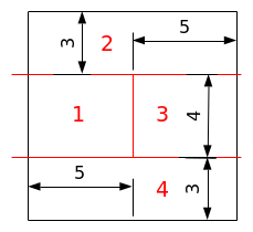
Figure 1.1-a: Structure geometry, interface position, and area numbering used to test the difference between calculated and analytical displacements.

1.2. Material properties

The material has an isotropic elastic behavior whose properties are as follows:

Young’s module: \(100\mathit{MPa}\)

Poisson’s ratio: \(0.3\)

1.3. Boundary conditions and loads

In the non-contact case (models A to E), moving conditions are applied on the left and right edges of the structure, so that each of the 4 zones formed by the interfaces has a different movement from the others according to \(\text{X}\). This load is shown in FIG. 1.3-a. We block the movements in \(\text{Y}\) (and in \(\text{Z}\) for 3D models) on these same edges.

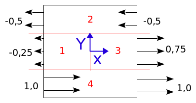
Figure 1.3-a: Illustration of boundary conditions and loads, non-contact cases.

In the case of contact (F to J models), roller conditions are imposed on the left and bottom edges, the stepped pressure in FIG. 1.3-b is applied to the right edge and a uniform pressure is applied to the top edge. This load is represented in FIG. 1.3-c. Each block is then compressed uniformly according to \(X\) and \(Y\). For \(\mathrm{3D}\) models, a roller condition is imposed in \(Z=0\).

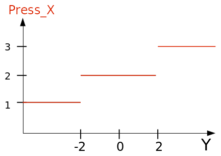
Figure 1.3-b: Pressure imposed along Y on the right edge, (in \(\text{[MPa]}\) ) .

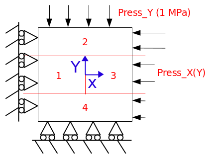
Figure 1.3-c: Illustration of boundary conditions and loads, contact cases.