1. Reference problem

1.1. Geometry

The structure is a healthy square in which two interfaces are introduced, shown in red in Figure 1.1-a. The two interfaces intersect. The dimensions of the structure as well as the position of the interfaces are given in this figure.

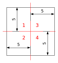
Figure 1.1-a: Structure geometry, interface position, and area numbering used to test the difference between calculated and analytical displacements.

1.2. Material properties

The material has an isotropic elastic behavior whose properties are:

Young’s module: \(100\mathit{MPa}\)

Poisson’s ratio: \(0.3\)

1.3. Boundary conditions and loads

In the non-contact case (models A to D), moving conditions are applied on the left and right edges of the structure, so that each of the 4 zones has a different displacement from the others according to \(X\). This load is shown in FIG. 1.3-a. We block the movements in \(Y\) (and in \(Z\) for the \(3D\) models) on these same edges. Rigid mode movements are then obtained for the 4 blocks.

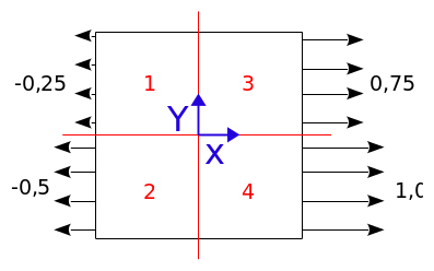
Figure 1.3-a: Illustration of boundary conditions and loads, non-contact cases.

In the case of contact (E to H models), roller conditions are imposed on the left and bottom edges and the stepped pressure in FIG. 1.3-b is applied to the right and top edges. This load is represented in FIG. 1.3-c. Each block is then compressed uniformly according to \(X\) and \(Y\). For \(\mathrm{3D}\) models, a roller condition is imposed in \(Z=0\).

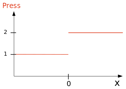
Figure 1.3-b: Pressure imposed along \(X\) on the top edge and according to \(Y\) on the right edge, (in \(\mathit{MPa}\) ) .

Figure 1.3-c: Illustration of boundary conditions and loads, contact cases.