6. D modeling#
6.1. Characteristics of modeling#
It is a modeling in plane deformations (D_ PLAN). The master and slave surfaces are not compliant.
Young’s modulus \({E}_{1}\mathrm{=}{E}_{2}\) and Poisson’s coefficients \({\nu }_{1}\mathrm{=}{\nu }_{2}\) are \(1.0E9\mathit{Pa}\) and \(0.2\) respectively. The pressure applied to the edge of the outer ring is \(1.0E7+\mathrm{10E5.cos}(2\theta )(\mathit{Pa})\), \(\theta\) being the polar angle.
The outer ring defines the master surface.
6.2. Characteristics of the mesh#
The mesh (Figure 4.2-1) includes:
480 SEG3 meshes;
2640 QUAD8 meshes.
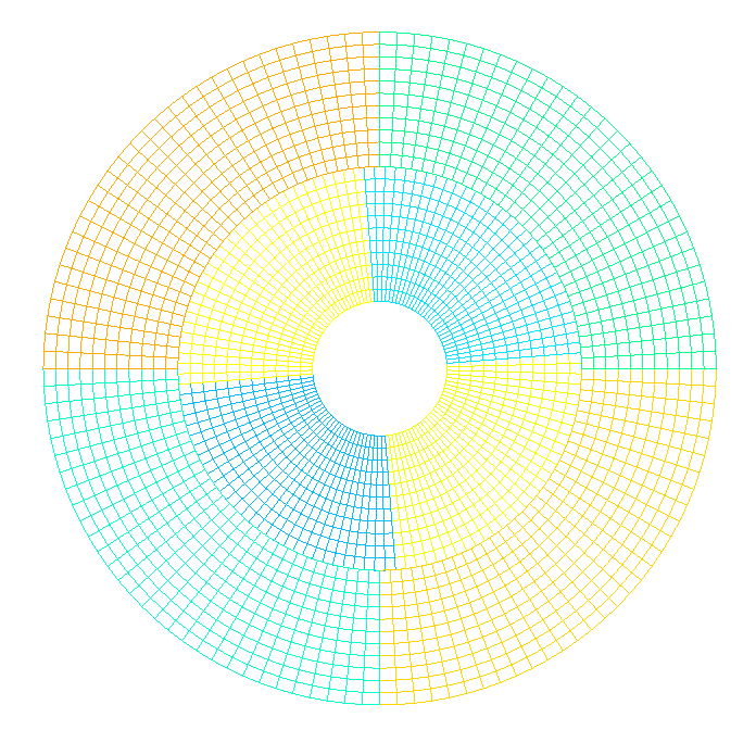
Figure 6.2-a : The D modeling mesh
6.3. Tested sizes and results#
Note \(\lambda\) the contact pressure calculated analytically, \(({U}_{x},{U}_{y})\) the displacements calculated analytically.
In the case where the displacements are zero, an absolute tolerance equal to 2% of the value of the maximum radial displacement Urmax=5.5E-03 is defined.
The contact pressure (LAGS_C) and the components of the displacement in the plane (X, Y) (DX, DY) are calculated for the nodes with the following coordinates:
N9 (5.98150400239877E-01, 4.70754574367070E-02)
N10 (-4.70754574367070E-02, 5.98150400239877E-01)
N11 (-5.98150400239877E-01, -4.70754574367070E-02)
N12 (4.70754574367070E-02, -5.98150400239877E-01)
N587 (3.89668829003112E-01, 4.56243579355747E-01)
N726 (-4.562435793579355747E-01, 3.89668829003112E-01)
N865 (-3.89668829003112E-01, -4.56243579355747E-01)
N1004 (4.562435793579355747E-01, -3.89668829003112E-01)
Identification |
Reference |
Aster |
tolerance |
LAGS_C at node 9 |
|
Analytics |
2.10-2 |
DX at node 9 |
|
Analytics |
2.10-2 |
DY at node 9 |
|
Analytics |
2.10-2 |
LAGS_C at node 10 |
|
Analytics |
2.10-2 |
DX at Node 10 |
|
Analytics |
2.10-2 |
DY at node 10 |
|
Analytics |
2.10-2 |
LAGS_C at node 11 |
|
Analytics |
2.10-2 |
DX at Node 11 |
|
Analytics |
2.10-2 |
DY at node 11 |
|
Analytics |
2.10-2 |
LAGS_C at node 12 |
|
Analytics |
2.10-2 |
DX at Node 12 |
|
Analytics |
2.10-2 |
DY at node 12 |
|
Analytics |
2.10-2 |
LAGS_C at node 587 |
|
Analytics |
2.10-2 |
DX at node 587 |
|
Analytics |
2.10-2 |
DY at node 587 |
|
Analytics |
2.10-2 |
LAGS_C at node 726 |
|
Analytics |
2.10-2 |
DX at node 726 |
|
Analytics |
2.10-2 |
DY at node 726 |
|
Analytics |
2.10-2 |
LAGS_C at node 865 |
|
Analytics |
2.10-2 |
DX at node 865 |
|
Analytics |
2.10-2 |
DY at node 865 |
|
Analytics |
2.10-2 |
LAGS_C at node 1004 |
|
Analytics |
2.10-2 |
DX at node 1004 |
|
Analytics |
2.10-2 |
DY at node 1004 |
|
Analytics |
2.10-2 |
Table 6.3-1