2. Benchmark solution#

2.1. General case#

In this part, we detail the analytical solution in pure \(I\) mode in its \(\mathrm{3D}\) form. For \(\mathrm{2D}\) plan calculations, the solution is the same. The jump component and the following stress vector \(\tau\) do not intervene, and it is enough to replace the surface \(S\) by the length \(L\) in the solution.

For loads in shear mode, the elastic element does not intervene.

Initially, the joint follows a round-trip loading in \(I\) mode, which makes it possible to test the profile of the force-displacement curve at various times for this type of loading. In the second part, we load sequentially in mode \(I\), then in mode \(\mathit{II}\) (or \(\mathit{III}\) depending on the modeling). Then we change the load to mode \(I\) and unload to mode \(\mathit{II}\). The coupling between the two loading modes is thus required (for example, it is verified that the tangential slope evolves according to normal loading). We also test the profile of the force-displacement curve for the tangential force.

2.2. In pure \(I\) mode#

The analytical solution of the global response of the system written in the local coordinate system \((n,t,\tau )\) is presented. We apply a loading collinear to the normal: \(U\mathrm{=}Un\), the cohesive element opens in pure \(I\) mode and the tangential constraints as well as the tangential jumps remain zero. So we are back to a scalar problem. We note \(\sigma \mathrm{=}n\mathrm{.}\sigma \mathrm{.}n\) the only non-zero component of the stress tensor of the elastic element in the local coordinate system:

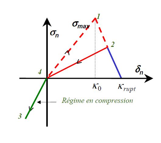
Figure 1: Roundtrip charging in \(I\) mode (law of JOINT_MECA_RUPT)

JOINT_MECA_RUPT

The solution of the global response of the join+cube system is presented (see document [R7.01.25]).

Equal constraints give:

\(\mathrm{\{}\begin{array}{c}\sigma \mathrm{=}{K}_{N}{\delta }_{n}\\ \sigma \mathrm{=}E{\varepsilon }_{\mathit{cube}}\mathrm{=}E(U\mathrm{-}{\delta }_{n})\mathrm{/}{L}_{\mathit{cube}}\end{array}\) in the elastic zone

\(\mathrm{\{}\begin{array}{c}\sigma \mathrm{=}{\sigma }_{\mathit{max}}\mathrm{-}{K}_{N}\mathrm{/}{P}_{\mathit{rup}}({\delta }_{n}\mathrm{-}{\sigma }_{\mathit{max}}\mathrm{/}{K}_{N})\\ \sigma \mathrm{=}E{\varepsilon }_{\mathit{cube}}\mathrm{=}E(U\mathrm{-}{\delta }_{n})\mathrm{/}{L}_{\mathit{cube}}\end{array}\) in the softening zone

Where \({L}_{\mathrm{cube}}=1\) is the length of the edge of the cube in our case. We note the maximum opening of the joint until complete rupture by \({U}_{\mathit{max}}\mathrm{=}{\sigma }_{\mathit{max}}(1+{P}_{\mathit{rup}})\mathrm{/}{K}_{N}\) and the maximum elastic opening by \({U}_{\mathit{el}}\mathrm{=}{\sigma }_{\mathit{max}}({K}_{N}{L}_{\mathit{cube}}+E)\mathrm{/}{K}_{N}E\).

The solution is given by the piecewise linear function:

\[\]

: label: EQ-None

< {U} _ {mathit {max}}\sigmamathrm {=} 0&text {si} & U>begin {array} {ccc}sigmamathrm {=}mathrm {=}}mathrm {-} {K} _ {N} {L} _ {L} _ {mathit {cube}} _ {mathit {cube}}}} +Emathrm {cube}}}} +Emathrm {cube}}} +Emathrm {-} {cube}}} +Emathrm {-} {cube}}} +Emathrm {-} {P} _ {mathit {cont}}} ({K} _ {N} {L}} _ {N} {L}} _ {N} {L}} _ {N} {L} _ {N} {L} _ {L} _ {\ sigmamathrm {=} {K} _ {N} _ {N} Emathrm {/} ({K} _ {N} {L} _ {mathit {cube}} +E) U&text {si}} & U< {U} & U< {U} _ {U} _ {U} _ {N} & U< {U} _ {U} _ {U} _ {U} _ {U} _ {U} _ {U} _ {U} _ {U} _ {U} _ {U} _ {U} _ {U} _ {U} _ {U} _ {U} _ {U} _ {U} _ {U} _ {U} _ {N} Emathrm {/}} (mathrm {-} {K} _ {N} {N} {L} _ {mathit {cube}}} +Emathrm {ast} {P} _ {mathit {rup}}) ({U} _ {mathit {max}}} {mathit {max}}}end {array}

The force tested is therefore given by \(F\mathrm{=}\sigma S\) where \(S\) corresponds to the surface on which the load is applied.

For hydro-mechanical models (G, H, I models) the force value is given by: \(F\mathrm{=}(\sigma \mathrm{-}{p}_{\mathit{fluide}})S\) where \({p}_{\mathit{fluide}}\) designates the pressure of the fluid contributing to the opening of the joint.

JOINT_MECA_FROT

The solution of the global response of the joint plus cube system is presented (see doc [R7.01.25]).

Equal constraints give:

\(\mathrm{\{}\begin{array}{c}\sigma \mathrm{=}c\mathrm{/}\mu \\ \sigma \mathrm{=}E{\varepsilon }_{\mathit{cube}}\mathrm{=}E(U\mathrm{-}{\delta }_{n})\mathrm{/}{L}_{\mathit{cube}}\end{array}\) in the plastic zone

Where \({L}_{\mathrm{cube}}=1\) is the length of the edge of the cube in our case. As the maximum stress in \(I\) mode for the Mohr-Coulomb law is given by \({\sigma }_{\mathit{max}}\mathrm{=}c\mathrm{/}\mu\), the maximum elastic opening (elastic traction threshold) is equal to \({U}_{\mathit{el}}\mathrm{=}{\sigma }_{\mathit{max}}({K}_{N}{L}_{\mathit{cube}}+E)\mathrm{/}{K}_{N}E\). We advance to this displacement value, we check the value of \(\sigma \mathrm{=}{\sigma }_{\mathit{max}}\mathrm{=}c\mathrm{/}\mu\), then we impose the double displacement and we check that the stress value does not change. Then, in the compression field, the solution is always elastic \(\sigma \mathrm{=}{K}_{N}{\delta }_{n}\).

The force tested is given by \(F\mathrm{=}\sigma S\) where \(S\) corresponds to the surface on which the load is applied.

For hydro-mechanical models (J, K, L models) the force value is given by: \(F\mathrm{=}(\sigma \mathrm{-}{p}_{\mathit{fluide}})S\) where \({p}_{\mathit{fluide}}\) designates the pressure of the fluid contributing to the opening of the joint.

2.3. In pure \(\mathit{II}\) and \(\mathit{III}\) mode#

The system written in the local coordinate system \((n,t,\tau )\). A loading perpendicular to the normal is applied directly to the joint: \(U\mathrm{=}{U}_{t}\tau\). The cohesive element opens in \(\mathit{II}\) mode. If normal loading does not change, we are back to a scalar problem. We note \({\sigma }_{n}\mathrm{=}n\mathrm{.}\sigma \mathrm{.}n\), \({\sigma }_{\tau }\mathrm{=}\tau \mathrm{.}\sigma \mathrm{.}n\) the constraints in the local coordinate system.

The loading in mode \(I\) being maintained, we load in mode \(\mathit{II}\) (or \(\mathit{III}\) depending on the model). The coupling between the two modes is thus required. The solution varies according to the law of behavior:

- JOINT_MECA_RUPT

When the joint is partially open (\({\delta }_{n}>0\)) the tangential slope evolves according to this normal opening as: \({K}_{T}^{\mathit{evol}}\mathrm{=}{K}_{T}\mathrm{\times }(1\mathrm{-}{\delta }_{n}\mathrm{/}{L}_{\mathit{CT}})\) (see doc [R7.01.25])

where \({L}_{\mathit{CT}}\mathrm{=}{\sigma }_{\mathit{max}}(1+{P}_{\mathit{rup}})\mathrm{/}{K}_{N}\mathrm{tan}(\alpha \pi \mathrm{/}4)\) is the critical tangential damage length. The solution is given by: \({\sigma }_{\tau }\mathrm{=}{K}_{T}^{\mathit{evol}}{U}_{t}\)

- JOINT_MECA_FROT

The force-displacement curve is tested for the joint, whose normal loading changes. The joint is partially closed (\({\delta }_{n}>0\)). The solution is the simple Mohr-Coulomb sliding. \({\sigma }_{\tau }\mathrm{=}\mathrm{-}\mu {\sigma }_{n}+c\) This curve is tested at various times (see illustration):

Illustration 2: Force (tangent) displacement curve for the JOINT_MECA_FROT law