1. Reference problem#
1.1. Geometry#
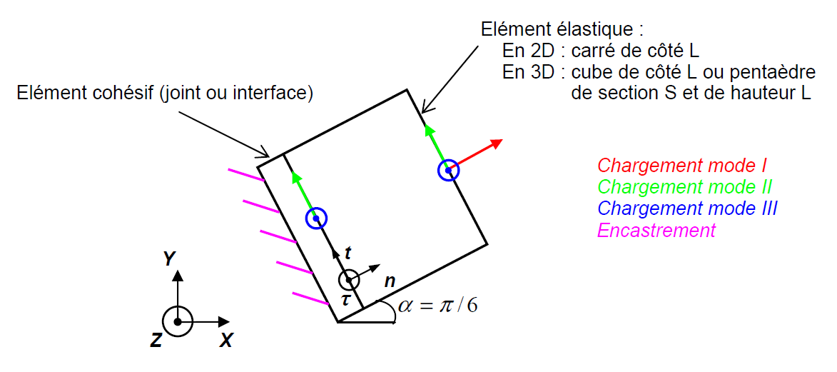
Figure 1: Representation of the system of two elements in the plane \((X,Y)\) .
We choose \(L=1\mathrm{mm}\).
1.2. Material properties#
1.2.1. Law JOINT_MECA_RUPT: material JOINT_MECA_RUPT#
**Cube:* elastic
Young’s module: \(E\mathrm{=}3\mathrm{\times }{10}^{12}\mathit{Pa}\)
Poisson’s ratio: \(\nu =0\)
normal stiffness: |
\({K}_{N}\mathrm{=}{10}^{12}\mathit{Pa}\mathrm{/}m\) |
(keyword: K_N) |
tangential stiffness: |
\({K}_{T}\mathrm{=}2\mathrm{\times }{10}^{12}\mathit{Pa}\mathrm{/}m\) |
(keyword: K_T) |
tensile strength: |
\({\sigma }_{\mathrm{max}}=0.1\mathrm{MPa}\) |
(keyword: SIGM_MAX) |
tangential damage control |
\(\alpha =1.5\) |
(keyword: ALPHA) |
fragile break smoothing parameter |
\({P}_{\mathrm{rup}}=0.5\) |
(keyword: PENA_RUPTURE) |
criminalization of contact |
\({P}_{\mathrm{cont}}=3\) |
(keyword: PENA_CONTACT) |
Fluid density (only for HM models) |
\({\rho }_{\mathrm{fluide}}=1000\mathrm{kg}/{m}^{3}\) |
(keyword: RHO_FLUIDE) |
Dynamic fluid viscosity (only for HM models) |
\({\mu }_{\mathrm{fluide}}=0.001\mathrm{Pa.s}\) |
(keyword: VISC_FLUIDE) |
Flow regulation opening (only for HM models) |
\({\delta }_{\mathrm{min}}=1.E-10m\) |
keyword: OUV_MIN) |
NB: Material data is of course not intended to represent a particular material. They are only intended for numerical validation tests.
1.2.2. Law JOINT_MECA_FROT: material JOINT_MECA_FROT#
**Cube:* elastic
Young’s module: \(E\mathrm{=}3\mathrm{\times }{10}^{12}\mathit{Pa}\)
Poisson’s ratio: \(\nu =0\)
normal stiffness: |
\({K}_{N}={10}^{12}\mathrm{Pa}/m\) |
(keyword: K_N) |
tangential stiffness: |
\({K}_{T}\mathrm{=}2\mathrm{\times }{10}^{12}\mathit{Pa}\mathrm{/}m\) |
(keyword: K_T) |
coefficient of friction: |
\(\mu =0.5\) |
(keyword: MU) |
adhesion (friction with zero normal loading) |
\(c={10}^{5}\mathrm{Pa}\) |
(keyword: ADHESION) |
regularization of the tangent slope while sliding |
\(\lambda ={10}^{-6}{K}_{T}\) |
(key word: PENA_TANG) |
NB: Material data is of course not intended to represent a particular material. They are only intended for numerical validation tests.
1.3. Boundary conditions and loads#
Embedment: The imposed displacements are zero on the face of the cohesive element opposite to the elastic element.
The joint is inclined at 30 degrees with respect to the horizontal plane, which gives the following directions of loading depending on the mode of stress:
In mode \(I\): An imposed displacement \(U\) is applied to the face of the elastic element opposite the joint (see figure 1).
\(\mathit{DX}\mathrm{=}2.16506351\) |
|
|
In mode \(\mathrm{II}\): The \(U\) imposed displacement is applied to all the nodes of the solid element.
\(\mathit{DX}\mathrm{=}\mathrm{-}1.250\) |
|
|
In mode \(\mathrm{III}\): The \(U\) imposed displacement is applied to all the nodes of the solid element.
\(\mathit{DX}\mathrm{=}0.0\) |
|
|
In \(I\) mode, the joint follows a loading pattern back and forth: first until the partial opening (\({\delta }_{n}>0\)), then it is compressed until \({\delta }_{n}<0\) and finally it is unloaded to its equilibrium point \({\delta }_{n}=0\).
In order to complete the mixed mode test we load partially in mode \(I\) and then we go back and forth in mode \(\mathrm{II}\) (or \(\mathrm{III}\) depending on the modeling).