2. Benchmark solution#

The reference solution for this test case is provided by the cohesive behavior relationship defined in [R7.02.12]:

\({t}_{c}=\frac{{\sigma }_{c}}{\alpha }\mathrm{exp}(\frac{-{\sigma }_{c}}{{G}_{c}}\alpha )({〚u〛}_{n}+{\beta }^{2}{〚u〛}_{\tau })\)

Where:

\(〚u〛\) is the move jump
\({〚u〛}_{n}=n\otimes n\mathrm{.}〚u〛\) is the projection of the jump movement following the normal one at the interface
\({〚u〛}_{\tau }=(\text{Id}-n\otimes n)\mathrm{.}〚u〛\) is the projection of the displacement jump along the tangential plane to the interface
\(\beta\) is a quantity obtained experimentally representing the ratio between the opening forces in Mode \(I\) and in Mode \(\mathrm{II}\). For this test, this parameter is chosen unitary.
\({〚u〛}_{\mathrm{eq}}=\sqrt{{∥{〚u〛}_{n}∥}^{2}+{\beta }^{2}{∥{〚u〛}_{\tau }∥}^{2}}\)
\(\alpha\) is an internal variable corresponding to the highest value of \({〚u〛}_{\mathrm{eq}}\) reached during the opening. This internal variable has the initial value \({\alpha }_{0}=\frac{{G}_{c}}{{\sigma }_{c}}\text{PENA\_ADHERENCE}\). If the material goes out of its elastic range, we have \(\alpha ={〚u〛}_{\mathrm{eq}}\).

We therefore know explicitly the cohesive force [1] _ depending on the movement jump.

Final calculation instant	Phase	Final move jump (in m)	\(\mid \mid {t}_{c}\mid \mid\) (in Pa)
0.5	Start of initial elastic load	2.73E-7	3.66296853301E+05
0.75	Initial Elastic Discharge	1.36E-7	1.8314842665E+05
2	End of initial elastic load	8,18E-7	1.098890559903E+06
3,5	Damage 1	1,50E-3	1.75867720687844E+05
4.5	Elastic discharge 1	5,00E-4	2.49999999999582E-04
5.5	Elastic load 1	1.50E-3	1.75867720687844E+05
7	Damage 2	3,00E-3	2.8117686527187E+04
9.5	Elastic discharge 2	5,00E-4	4.68628108785798E+03
12	Elastic load 2	3,00E-3	2.8117686527187E+04
15	Damage 3	6,00E-3	7.18731177854856E+02

This value will therefore be compared to the contact and friction values of the Lagrangians, respectively named LAGS_C and LAGS_F1.

Fashion \(I\) :

For reasons of invariance, let us consider a one-dimensional problem. We will also assume that the structure is meshed with only three elements, which does not change the validity of the results stated later. The interface is present in the middle of the central element as shown in []. Since we DDL_IMPO control the \(\mathrm{H1Y}\) degree of freedom of node \(\text{N2}\) (also noted as \({b}_{\mathrm{y2}}\)), let’s solve the problem based on this parameter.

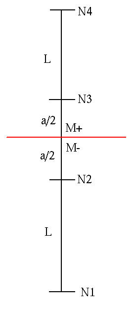
Figure 2-a : One-dimensional representation of the reference problem

Let us express the movements of the different points of the structure:

\(\mathrm{\{}\begin{array}{c}{u}^{1}\mathrm{=}0\\ {u}^{2}\mathrm{=}L\epsilon \\ {u}^{\text{+}}\mathrm{=}(L+\frac{a}{2})\epsilon \\ {u}^{\text{-}}\mathrm{=}(L+\frac{a}{2})\epsilon +{\mathrm{[}\mathrm{[}u\mathrm{]}\mathrm{]}}_{n}\\ {u}^{3}\mathrm{=}(L+a)\epsilon +{\mathrm{[}\mathrm{[}u\mathrm{]}\mathrm{]}}_{n}\\ {u}^{4}\mathrm{=}(\mathrm{2L}+a)\epsilon +{\mathrm{[}\mathrm{[}u\mathrm{]}\mathrm{]}}_{n}\end{array}\)

Now let’s express the displacements of the points \(\text{N2}\), \(\text{M+}\),, \(\text{M-}\), and \(\text{N3}\) according to the degrees of freedom \(X-\mathrm{FEM}\).

\(\mathrm{\{}\begin{array}{c}{u}^{2}\mathrm{=}{a}_{\mathit{y2}}\mathrm{-}{b}_{\mathit{y2}}\\ {u}^{3}\mathrm{=}{a}_{\mathit{y2}}+{b}_{\mathit{y3}}\\ {u}^{\text{+}}\mathrm{=}\frac{{a}_{\mathit{y2}}+{b}_{\mathit{y2}}}{2}+\frac{{a}_{\mathit{y3}}+{b}_{\mathit{y3}}}{2}\\ {u}^{\text{-}}\mathrm{=}\frac{{a}_{\mathit{y2}}\mathrm{-}{b}_{\mathit{y2}}}{2}+\frac{{a}_{\mathit{y3}}\mathrm{-}{b}_{\mathit{y3}}}{2}\end{array}\)

By inverting this system, we obtain:

\(\mathrm{\{}\begin{array}{c}{a}_{\mathit{y2}}\mathrm{=}\frac{{u}_{2}}{2}\mathrm{-}\frac{{u}_{3}}{2}+{u}^{\text{+}}\\ {b}_{\mathit{y2}}\mathrm{=}\mathrm{-}\frac{{u}_{2}}{2}\mathrm{-}\frac{{u}_{3}}{2}+{u}^{\text{+}}\\ {a}_{\mathit{y3}}\mathrm{=}\mathrm{-}\frac{{u}_{2}}{2}+\frac{{u}_{3}}{2}+{u}^{\text{-}}\\ {b}_{\mathit{y3}}\mathrm{=}\frac{{u}_{2}}{2}+\frac{{u}_{3}}{2}\mathrm{-}{u}^{\text{-}}\end{array}\)

The elastic law of structure gives: \(\sigma =E\epsilon\).

The balance of the system gives \(\sigma ={t}_{c}\).

Finally, the law of cohesive behavior provides a relationship between stress and displacement jump. This relationship is different depending on whether the joint remains in its elastic domain or if it is damaged.

If the joint remains in the elastic domain, the internal variable \(\alpha\) remains constant. So we have \({t}_{c}=\frac{{\sigma }_{c}}{\alpha }\mathrm{exp}(\frac{-{\sigma }_{c}}{{G}_{c}}\alpha ){〚u〛}_{n}\).

The movements of the various points of the structure are then written as:

\(\mathrm{\{}\begin{array}{c}{u}^{1}\mathrm{=}0\\ {u}^{2}\mathrm{=}\frac{L}{E}\frac{{\sigma }_{c}}{\alpha }\mathrm{exp}(\frac{\mathrm{-}{\sigma }_{c}}{{G}_{c}}\alpha ){\mathrm{〚}u\mathrm{〛}}_{n}\\ {u}^{\text{+}}\mathrm{=}\frac{L+\frac{a}{2}}{E}\frac{{\sigma }_{c}}{\alpha }\mathrm{exp}(\frac{\mathrm{-}{\sigma }_{c}}{{G}_{c}}\alpha ){\mathrm{〚}u\mathrm{〛}}_{n}\\ {u}^{\text{-}}\mathrm{=}(1+\frac{L+\frac{a}{2}}{E}\frac{{\sigma }_{c}}{\alpha }\mathrm{exp}(\frac{\mathrm{-}{\sigma }_{c}}{{G}_{c}}\alpha )){\mathrm{〚}u\mathrm{〛}}_{n}\\ {u}^{3}\mathrm{=}(1+\frac{L+a}{E}\frac{{\sigma }_{c}}{\alpha }\mathrm{exp}(\frac{\mathrm{-}{\sigma }_{c}}{{G}_{c}}\alpha )){\mathrm{〚}u\mathrm{〛}}_{n}\\ {u}^{4}\mathrm{=}(1+\frac{\mathrm{2L}+a}{E}\frac{{\sigma }_{c}}{\alpha }\mathrm{exp}(\frac{\mathrm{-}{\sigma }_{c}}{{G}_{c}}\alpha )){\mathrm{〚}u\mathrm{〛}}_{n}\end{array}\)

By injecting these expressions into the formulas giving \({b}_{\mathrm{y2}}\) and \({b}_{\mathrm{y3}}\), we see that \({b}_{\mathrm{y2}}={b}_{\mathrm{y3}}\).

So we have \({[[u]]}_{n}={u}^{\text{+}}-{u}^{\text{-}}={b}_{\mathrm{y2}}+{b}_{\mathrm{y3}}={\mathrm{2.b}}_{\mathrm{y2}}\). The problem is therefore entirely determined for the given degree of freedom \({b}_{\mathrm{y2}}\), corresponding to the half-jump in movement, and known at all times thanks to piloting.

If the joint remains in the damage phase, the internal variable \(\alpha\) becomes equal to the displacement jump \({[[u]]}_{n}\). So we have \({t}_{c}\mathrm{=}{\sigma }_{c}\mathrm{exp}(\frac{\mathrm{-}{\sigma }_{c}}{{G}_{c}}{\mathrm{〚}u\mathrm{〛}}_{n})\).

The movements of the various points of the structure are then written as:

\(\mathrm{\{}\begin{array}{c}{u}^{1}\mathrm{=}0\\ {u}^{2}\mathrm{=}\frac{L}{E}{\sigma }_{c}\mathrm{exp}(\frac{\mathrm{-}{\sigma }_{c}}{{G}_{c}}{\mathrm{〚}u\mathrm{〛}}_{n})\\ {u}^{\text{+}}\mathrm{=}\frac{L+\frac{a}{2}}{E}{\sigma }_{c}\mathrm{exp}(\frac{\mathrm{-}{\sigma }_{c}}{{G}_{c}}{\mathrm{〚}u\mathrm{〛}}_{n})\\ {u}^{\text{-}}\mathrm{=}\frac{(L+\frac{a}{2})}{E}{\sigma }_{c}\mathrm{exp}(\frac{\mathrm{-}{\sigma }_{c}}{{G}_{c}}{\mathrm{〚}u\mathrm{〛}}_{n})+{\mathrm{[}\mathrm{[}u\mathrm{]}\mathrm{]}}_{n}\\ {u}^{3}\mathrm{=}\frac{(L+a)}{E}{\sigma }_{c}\mathrm{exp}(\frac{\mathrm{-}{\sigma }_{c}}{{G}_{c}}{\mathrm{〚}u\mathrm{〛}}_{n})+{\mathrm{[}\mathrm{[}u\mathrm{]}\mathrm{]}}_{n}\\ {u}^{4}\mathrm{=}\frac{(\mathrm{2L}+a)}{E}{\sigma }_{c}\mathrm{exp}(\frac{\mathrm{-}{\sigma }_{c}}{{G}_{c}}{\mathrm{〚}u\mathrm{〛}}_{n})+{\mathrm{[}\mathrm{[}u\mathrm{]}\mathrm{]}}_{n}\end{array}\)

By injecting these expressions into the formulas giving \({b}_{\mathit{y2}}\) and \({b}_{\mathit{y3}}\), we see that \({b}_{\mathit{y2}}\mathrm{=}{b}_{\mathit{y3}}\).

So we have \({\mathrm{[}\mathrm{[}u\mathrm{]}\mathrm{]}}_{n}\mathrm{=}{u}^{\text{+}}\mathrm{-}{u}^{\text{-}}\mathrm{=}{b}_{\mathit{y2}}+{b}_{\mathit{y3}}\mathrm{=}{\mathrm{2.b}}_{\mathit{y2}}\). The problem is therefore entirely determined for the given degree of freedom \({b}_{\mathit{y2}}\), corresponding to the half-jump in movement, and known at all times thanks to piloting.

Fashion \(\mathrm{II}\) :

The boundary conditions and relationships imposed thanks to the keyword factor LIAISON_GROUP ensure perfect shear at the interface level. The displacement of all the points located under the level set is therefore zero and the displacement of all the points located above the level set is equal to the movement jump.

The cohesive force in the joint is therefore known as an explicit function of the displacement jump, which is itself known at all times thanks to control.